Jdtcujk

Mapping that associates a single output value to each input

In mathematics, a function^[1] was originally the idealization of how a varying quantity depends on another quantity. For example, the position of a planet is a function of time. Historically, the concept was elaborated with the infinitesimal calculus at the end of the 17th century, and, until the 19th century, the functions that were considered were differentiable (that is, they had a high degree of regularity). The concept of function was formalized at the end of the 19th century in terms of set theory, and this greatly enlarged the domains of application of the concept.

A function is a process or a relation that associates each element $x$ of a set $X$ , the domain of the function, to a single element $y$ of another set $Y$ (possibly the same set), the codomain of the function. If the function is called $f$ , this relation is denoted $y = f (x)$ (read $f$ of $x$ ), the element $x$ is the argument or input of the function, and $y$ is the value of the function, the output, or the image of $x$ by $f$ .^[2] The symbol that is used for representing the input is the variable of the function (one often says that $f$ is a function of the variable $x$ ).

A function is uniquely represented by its graph which is the set of all pairs $(x, f (x))$ . When the domain and the codomain are sets of numbers, each such pair may be considered as the Cartesian coordinates of a point in the plane. In general, these points form a curve, which is also called the graph of the function. This is a useful representation of the function, which is commonly used everywhere. For example, graphs of functions are commonly used in newspapers for representing the evolution of price indexes and stock market indexes

Functions are widely used in science, and in most fields of mathematics. Their role is so important that it has been said that they are "the central objects of investigation" in most fields of mathematics.^[3]

Schematic depiction of a function described metaphorically as a "machine" or "black box" that for each input yields a corresponding output

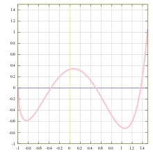
The red curve is the graph of a function, because any vertical line has exactly one crossing point with the curve.

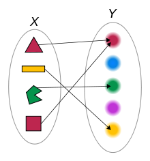
A function that associates any of the four colored shapes to its color.

Definition

.mw-parser-output .tmulti .thumbinner{display:flex;flex-direction:column}.mw-parser-output .tmulti .trow{display:flex;flex-direction:row;clear:left;flex-wrap:wrap;width:100%;box-sizing:border-box}.mw-parser-output .tmulti .tsingle{margin:1px;float:left}.mw-parser-output .tmulti .theader{clear:both;font-weight:bold;text-align:center;align-self:center;background-color:transparent;width:100%}.mw-parser-output .tmulti .thumbcaption{text-align:left;background-color:transparent}.mw-parser-output .tmulti .text-align-left{text-align:left}.mw-parser-output .tmulti .text-align-right{text-align:right}.mw-parser-output .tmulti .text-align-center{text-align:center}@media all and (max-width:720px){.mw-parser-output .tmulti .thumbinner{width:100%!important;box-sizing:border-box;max-width:none!important;align-items:center}.mw-parser-output .tmulti .trow{justify-content:center}.mw-parser-output .tmulti .tsingle{float:none!important;max-width:100%!important;box-sizing:border-box;text-align:center}.mw-parser-output .tmulti .thumbcaption{text-align:center}}

Diagram of a function, with domain X={1, 2, 3} and codomain Y={A, B, C, D}, which is defined by the set of ordered pairs {(1,D), (2,C), (3,C)}. The image/range is the set {C,D}.

This diagram, representing the set of pairs {(1,D), (2,B), (2,C)}, does not define a function. One reason is that 2 is the first element in more than one ordered pair, (2, B) and (2, C), of this set. Two other reasons, also sufficient by themselves, is that neither 3 nor 4 are first elements (input) of any ordered pair therein.

Intuitively, a function is a process that associates to each element of a set $X$ a single element of a set $Y$ .

Formally, a function $f$ from a set $X$ to a set $Y$ is defined by a set $G$ of ordered pairs $(x, y)$ such that $x \in X$ , $y \in Y$ , and every element of $X$ is the first component of exactly one ordered pair in $G$ .^[4]^{[note 1]} In other words, for every $x$ in $X$ , there is exactly one element $y$ such that the ordered pair $(x, y)$ belongs to the set of pairs defining the function $f$ . The set $G$ is called the graph of the function. Formally speaking, it may be identified with the function, but this hides the usual interpretation of a function as a process. Therefore, in common usage, the function is generally distinguished from its graph. Functions are also called maps or mappings, though some authors make some distinction between "maps" and "functions" (see #Map vs function).

In the definition of function, $X$ and $Y$ are respectively called the domain and the codomain of the function $f$ . If $(x, y)$ belongs to the set defining $f$ , then $y$ is the image of $x$ under $f$ , or the value of $f$ applied to the argument $x$ . Especially in the context of numbers, one says also that $y$ is the value of $f$ for the value $x$ of its variable, or, still shorter, $y$ is the value of $f$ of $x$ , denoted as $y = f (x)$ .

Two functions $f$ and $g$ are equal if their domain and codomain sets are the same and their output values agree on the whole domain. Formally, $f = g$ if $f (x) = g (x)$ for all $x \in X$ , where $f : X \to Y$ and $g : X \to Y$ .^[5]^[6]^{[note 2]}

The domain and codomain are not always explicitly given when a function is defined, and, without some (possibly difficult) computation, one knows only that the domain is contained in a larger set. Typically, this occurs in mathematical analysis, where "a function from $X$ to $Y$ " often refers to a function that may have a proper subset of $X$ as domain. For example, a "function from the reals to the reals" may refer to a real-valued function of a real variable, and this phrase does not mean that the domain of the function is the whole set of the real numbers, but only that the domain is a set of real numbers that contains a non-empty open interval; such a function is then called a partial function. For example, if $f$ is a function that has the real numbers as domain and codomain, then a function mapping the value $x$ to the value ${displaystyle g(x)={tfrac {1}{f(x)}}}$ is a function $g$ from the reals to the reals, whose domain is the set of the reals $x$ , such that $f (x) \neq 0$ .

The range of a function is the set of the images of all elements in the domain. However, range is sometimes used as a synonym of codomain, generally in old textbooks.^{[citation needed]}

Relational approach

Any subset of the Cartesian product of a domain $X$ and a codomain $Y$ is said to define a binary relation ${displaystyle Rsubseteq (Xtimes Y)}$ between these two sets. It is immediate that an arbitrary relation may contain pairs that violate the necessary conditions for a function, given above.

A univalent relation is a relation such that

{displaystyle (x,y)in R;land ;(x,z)in Rquad Rightarrow quad y=z.}

Univalent relations may be identified to functions whose domain is a subset of $X$ .

A left-total relation is a relation such that

{displaystyle forall xin X;exists yin Ycolon (x,y)in R.}

Formally, functions may be identified to relations that are both univalent and left total. Violating the left-totality is similar to giving a convenient encompassing set instead of the true domain, as explained above.

Various properties of functions and function composition may be reformulated in the language of relations. For example, a function is injective if the converse relation ${displaystyle R^{text{T}}subseteq (Ytimes X)}$ is univalent, where the converse relation is defined as ${displaystyle R^{text{T}}={(y,x):(x,y)in R}.}$ ^[7]

As an element of a Cartesian product over a domain

The set of all functions from some given domain to a codomain is sometimes identified with the Cartesian product of copies of the codomain, indexed by the domain. Namely, given sets $X,Y$ , any function $f:Xto Y$ is an element of the Cartesian product of copies of $Y$ 's over the index set $X$

{displaystyle fin prod _{X}Y=Y^{X}.}

Viewing $f$ as tuple with coordinates, then for each $xin X$ , the x-th coordinate of this tuple is the value ${displaystyle f(x)in Y.}$ This reflects the intuition that for each ${displaystyle xin X,}$ the function picks some element ${displaystyle yin Y,}$ namely, $f(x)$ . (This point of view is used for example in the discussion of a choice function.)

Note: infinite Cartesian products are often simply "defined" as sets of functions.^[8]

Notation

There are various standard ways for denoting functions. The most commonly used notation is functional notation, which defines the function using an equation that gives the names of the function and the argument explicitly. This gives rise to a subtle point, often glossed over in elementary treatments of functions: functions are distinct from their values. Thus, a function $f$ should be distinguished from its value $f (x 0)$ at the value $x 0$ in its domain. To some extent, even working mathematicians will conflate the two in informal settings for convenience, and to avoid the use of pedantic language. However, strictly speaking, it is an abuse of notation to write "let ${displaystyle fcolon mathbb {R} to mathbb {R} }$ be the function $f (x) = x 2$ ", since $f (x)$ and $x 2$ should both be understood as the value of f at x, rather than the function itself. Instead, it is correct, though pedantic, to write "let ${displaystyle fcolon mathbb {R} to mathbb {R} }$ be the function defined by the equation $f (x) = x 2,$ valid for all real values of $x$ ".

This distinction in language and notation becomes important in cases where functions themselves serve as inputs for other functions. (A function taking another function as an input is termed a functional.) Other approaches to denoting functions, detailed below, avoid this problem but are less commonly used.

Functional notation

As first used by Leonhard Euler in 1734,^[9] functions are denoted by a symbol consisting generally of a single letter in italic font, most often the lower-case letters $f, g, h$ . Some widely used functions are represented by a symbol consisting of several letters (usually two or three, generally an abbreviation of their name). By convention, in this case, a roman type is used, such as " $sin$ " for the sine function, in contrast to italic font for single-letter symbols.

The notation (read: " $y$ equals $f$ of $x$ ")

y=f(x)

means that the pair $(x, y)$ belongs to the set of pairs defining the function $f$ . If $X$ is the domain of $f$ , the set of pairs defining the function is thus, using set-builder notation,

{displaystyle {(x,f(x)):xin X}.}

Often, a definition of the function is given by what f does to the explicit argument x. For example, a function f can be defined by the equation

{displaystyle f(x)=sin(x^{2}+1)}

for all real numbers x. In this example, f can be thought of as the composite of several simpler functions: squaring, adding 1, and taking the sine. However, only the sine function has a common explicit symbol (sin), while the combination of squaring and then adding 1 is described by the polynomial expression $x^{2}+1$ . In order to explicitly reference functions such as squaring or adding 1 without introducing new function names (e.g., by defining function g and h by $g(x)=x^{2}$ and ${displaystyle h(x)=x+1}$ ), one of the methods below (arrow notation or dot notation) could be used.

Sometimes the parentheses of functional notation are omitted when the symbol denoting the function consists of several characters and no ambiguity may arise. For example, $sin x$ can be written instead of ${displaystyle sin(x).}$

Arrow notation

For explicitly expressing domain $X$ and the codomain $Y$ of a function $f$ , the arrow notation is often used (read: "the function $f$ from $X$ to $Y$ " or "the function $f$ mapping elements of $X$ to elements of $Y$ "):

fcolon Xto Y

or

{displaystyle X~{stackrel {f}{to }}~Y.}

This is often used in relation with the arrow notation for elements (read: " $f$ maps $x$ to $f (x)$ "), often stacked immediately below the arrow notation giving the function symbol, domain, and codomain:

{displaystyle xmapsto f(x).}

For example, if a multiplication is defined on a set $X$ , then the square function ${displaystyle operatorname {sqr} }$ on $X$ is unambiguously defined by (read: "the function ${displaystyle operatorname {sqr} }$ from $X$ to $X$ that maps $x$ to $x \cdot x$ ")

{displaystyle {begin{aligned}operatorname {sqr} colon X&to X\x&mapsto xcdot x,end{aligned}}}

the latter line being more commonly written

{displaystyle xmapsto x^{2}.}

Often, the expression giving the function symbol, domain and codomain is omitted. Thus, the arrow notation is useful for avoiding introducing a symbol for a function that is defined, as it is often the case, by a formula expressing the value of the function in terms of its argument. As a common application of the arrow notation, suppose ${displaystyle fcolon Xtimes Xto Y;;(x,t)mapsto f(x,t)}$ is a two-argument function, and we want to refer to a partially applied function $Xto Y$ produced by fixing the second argument to the value $t 0$ without introducing a new function name. The map in question could be denoted ${displaystyle xmapsto f(x,t_{0})}$ using the arrow notation for elements. Note that the expression ${displaystyle xmapsto f(x,t_{0})}$ (read: "the map taking $x$ to ${displaystyle f(x,t_{0})}$ ") represents this new function with just one argument, whereas the expression ${displaystyle f(x_{0},t_{0})}$ refers to the value of the function $f$ at the point ${displaystyle (x_{0},t_{0})}$ .

Index notation

Index notation is often used instead of functional notation. That is, instead of writing $f (x)$ , one writes ${displaystyle f_{x}.}$

This is typically the case for functions whose domain is the set of the natural numbers. Such a function is called a sequence, and, in this case the element $f_{n}$ is called the $n$ th element of sequence.

The index notation is also often used for distinguishing some variables called parameters from the "true variables". In fact, parameters are specific variables that are considered as being fixed during the study of a problem. For example, the map ${displaystyle xmapsto f(x,t)}$ (see above) would be denoted $f_{t}$ using index notation, if we define the collection of maps $f_{t}$ by the formula ${displaystyle f_{t}(x)=f(x,t)}$ for all ${displaystyle x,tin X}$ .

Dot notation

In the notation
${displaystyle xmapsto f(x),}$
the symbol $x$ does not represent any value, it is simply a placeholder meaning that, if $x$ is replaced by any value on the left of the arrow, it should be replaced by the same value on the right of the arrow. Therefore, $x$ may be replaced by any symbol, often an interpunct " $\cdot$ ". This may be useful for distinguishing the function $f (\cdot)$ from its value $f (x)$ at $x$ .

For example, ${displaystyle a(cdot )^{2}}$ may stand for the function ${displaystyle xmapsto ax^{2}}$ , and ${displaystyle textstyle int _{a}^{,(cdot )}f(u),du}$ may stand for a function defined by an integral with variable upper bound: ${displaystyle textstyle xmapsto int _{a}^{x}f(u),du}$ .

Specialized notations

There are other, specialized notations for functions in sub-disciplines of mathematics. For example, in linear algebra and functional analysis, linear forms and the vectors they act upon are denoted using a dual pair to show the underlying duality. This is similar to the use of bra–ket notation in quantum mechanics. In logic and the theory of computation, the function notation of lambda calculus is used to explicitly express the basic notions of function abstraction and application. In category theory and homological algebra, networks of functions are described in terms of how they and their compositions commute with each other using commutative diagrams that extend and generalize the arrow notation for functions described above.

Map vs function

A function is often also called a map or a mapping. But some authors make a distinction between the term "map" and "function". For example, the term "map" is often reserved for a "function" with some sort of special structure; e.g., a group homomorphism between groups can simply be called a map between those groups for the sake of succinctness. See also: maps of manifolds. Some authors^[10] reserve the word mapping to the case where the codomain Y belongs explicitly to the definition of the function. In this sense, the graph of the mapping recovers the function as the set of pairs.

Because the term "map" is synonymous with "morphism" in category theory, the term "map" can in particular emphasize the aspect that a function is a morphism in the category of sets: in the informal definition of function $f:Xto Y$ , it is a subset of $Xtimes Y$ consisting of all the pairs $(x,f(x))$ for $xin X$ . In this sense, the function doesn't capture the information of which set $Y$ is used as the co-domain. Only the range $f(X)$ is determined by the function.

Some authors, such as Serge Lang,^[11] use "function" only to refer to maps in which the codomain is a set of numbers (i.e. a subset of the fields R or C) and the term mapping for more general functions.

In the theory of dynamical systems, a map denotes an evolution function used to create discrete dynamical systems. See also Poincaré map.

A partial map is a partial function, and a total map is a total function. Related terms like domain, codomain, injective, continuous, etc. can be applied equally to maps and functions, with the same meaning. All these usages can be applied to "maps" as general functions or as functions with special properties.

Specifying a function

Given a function $f$ , by definition, to each element $x$ of the domain of the function $f$ , there is a unique element associated to it, the value $f(x)$ of $f$ at $x$ . There are several ways to specify or describe how $x$ is related to $f(x)$ , both explicitly and implicitly. Sometimes, a theorem or an axiom asserts the existence of a function having some properties, without describing it more precisely. Often, the specification or description is referred to as the definition of the function $f$ .

By listing function values

On a finite set, a function may be defined by listing the elements of the codomain that are associated to the elements of the domain. E.g., if ${displaystyle A={1,2,3}}$ , then one can define a function $f:Ato {mathbb {R}}$ by ${displaystyle f(1)=2,f(2)=3,f(3)=4.}$

By a formula

Functions are often defined by a formula that describes a combination of arithmetic operations and previously defined functions; such a formula allows computing the value of the function from the value of any element of the domain.
For example, in the above example, $f$ can be defined by the formula ${displaystyle f(n)=n+1}$ , for ${displaystyle nin {1,2,3}}$ .

When a function is defined this way, the determination of its domain is sometimes difficult. If the formula that defines the function contains divisions, the values of the variable for which a denominator is zero must be excluded from the domain; thus, for a complicated function, the determination of the domain passes through the computation of the zeros of auxiliary functions. Similarly, if square roots occur in the definition of a function from $mathbb {R}$ to ${displaystyle mathbb {R} ,}$ the domain is included in the set of the values of the variable for which the arguments of the square roots are nonnegative.

For example, ${displaystyle f(x)={sqrt {1+x^{2}}}}$ defines a function $f:{mathbb {R}}to {mathbb {R}}$ whose domain is ${displaystyle mathbb {R} ,}$ because ${displaystyle 1+x^{2}}$ is always positive if $x$ is a real number. On the other hand, $f(x)=sqrt{1-x^2}$ defines a function from the reals to the reals whose domain is reduced to the interval $[-1, 1]$ . (In old texts, such a domain was called the domain of definition of the function.)

Function are often classified by the nature of formulas that can that define them:

A quadratic function is a function that may be written ${displaystyle f(x)=ax^{2}+bx+c,}$ where $a, b, c$ are constants.

More generally, a polynomial function is a function that can be defined by a formula involving only additions, subtractions, multiplications, and exponentiation to nonnegative integers. For example, ${displaystyle f(x)=x^{3}-3x-1,}$ and ${displaystyle f(x)=(x-1)(x^{3}+1)+2x^{2}-1.}$

A rational function is the same, with divisions also allowed, such as ${displaystyle f(x)={frac {x-1}{x+1}},}$ and ${displaystyle f(x)={frac {1}{x+1}}+{frac {3}{x}}-{frac {2}{x-1}}.}$

An algebraic function is the same, with $n$ th roots and roots of polynomials also allowed.

An elementary function^{[note 3]} is the same, with logarithms and exponential functions allowed.

Inverse and implicit functions

A function ${displaystyle f:Xto Y,}$ with domain $X$ and codomain $Y$ , is bijective, if for every $y$ in $Y$ , there is one and only one element $x$ in $Y$ such that $y = f (x)$ . In this case, the inverse function of $f$ is the function ${displaystyle f^{-1}:Yto X}$ that maps $yin Y$ to the element $xin X$ such that $y = f (x)$ . For example, the natural logarithm is a bijective function from the positive real numbers to the real numbers. It has these an inverse, called the exponential function that maps the real numbers onto the positive numbers.

If a function $f:Xto Y$ is not bijective, it may occur that one can select subsets ${displaystyle Esubseteq X}$ and ${displaystyle Fsubseteq Y}$ such that the restriction of $f$ to $E$ is a bijection from $E$ to $F$ , and has thus an inverse. The inverse trigonometric functions are defined this way. For example, the cosine function induces, by restriction, a bijection from the interval $[0, π]$ onto the interval $[-1, 1]$ , and its inverse function, called arccosine, maps $[-1, 1]$ onto $[0, π]$ . The other inverse trigonometric functions are defined similarly.

More generally, given a binary relation $R$ between two sets $X$ and $Y$ , let $E$ be a subset of $X$ such that, for every ${displaystyle xin E,}$ there is some $yin Y$ such that $x R y$ . If one has a criterion allowing selecting such an $y$ for every ${displaystyle xin E,}$ this defines a function ${displaystyle f:Eto Y,}$ called an implicit function, because it is implicitly defined by the relation $R$ .

For example, the equation of the unit circle $x^{2}+y^{2}=1$ defines a relation on real numbers. If $-1 < x < 1$ there are two possible values of $y$ , one positive and one negative. For $x = \pm 1$ , these two values become both equal to 0. Otherwise, there is no possible value of $y$ . This means that the equation defines two implicit functions with domain $[-1, 1]$ and respective codomains $[0, +\infty)$ and $(-\infty, 0]$ .

In this example, the equation can be solved in $y$ , giving ${displaystyle y=pm {sqrt {1-x^{2}}},}$ but, in more complicated examples, this is impossible. For example, the relation ${displaystyle y^{5}+x+1=0}$ defines $y$ as an implicit function of $x$ , called the Bring radical, which has $mathbb {R}$ as domain and range. The Bring radical cannot be expressed in terms of the four arithmetic operations and $n$ th roots.

The implicit function theorem provides mild differentiability conditions for existence and uniqueness of an implicit function in the neighborhood of a point.

Using differential calculus

Many functions can be defined as the antiderivative of another function. This is the case of the natural logarithm, which is the antiderivative of $1/ x$ that is 0 for $x = 1$ . An other common example is the error function.

More generally, many functions, including most special functions, can be defined as solutions of differential equations. The simplest example is probably the exponential function, which can be defined as the unique function that is equal to its derivative and takes the value 1 for $x = 0$ .

Power series can be used to define functions on the domain in which they converge. For example, the exponential function is given by ${displaystyle e^{x}=sum _{n=0}^{infty }{x^{n} over n!}}$ . However, as the coefficients of a series are quite arbitrary, a function that is the sum of a convergent series is generally defined otherwise, and the sequence of the coefficients is the result of some computation based on another definition. Then, the power series can be used to enlarge the domain of the function. Typically, if a function for a real variable is the sum of its Taylor series in some interval, this power series allows immediately enlarging the domain to a subset of the complex numbers, the disc of convergence of the series. Then analytic continuation allows enlarging further the domain for including almost the whole complex plane. This process is the method that is generally used for defining the logarithm, the exponential and the trigonometric functions of a complex number.

By recurrence

Functions whose domain are the nonnegative integers, known as sequences, are often defined by recurrence relations.

The factorial function on the nonnegative integers ( ${displaystyle nmapsto n!}$ ) is a basic example, as it can be defined by the recurrence relation

{displaystyle n!=n(n-1)!quad {text{for}}quad n>0,}

and the initial condition

{displaystyle 0!=1.}

Representing a function

A graph is commonly used to give an intuitive picture of a function. As an example of how a graph helps understand a function, it is easy to see from its graph whether a function is increasing or decreasing. Some functions may also be represented by bar charts.

Graphs and plots

The function mapping each year to its US motor vehicle death count, shown as a line chart

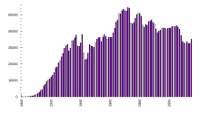
The same function, shown as a bar chart

Given a function ${displaystyle fcolon Xto Y,}$ its graph is, formally, the set

{displaystyle G={(x,f(x)):xin X}.}

In the frequent case where $X$ and $Y$ are subsets of the real numbers (or may be identified with such subsets, e.g. intervals), an element ${displaystyle (x,y)in G}$ may be identified with a point having coordinates $x, y$ in a 2-dimensional coordinate system, e.g. the Cartesian plane. Parts of this may create a plot that represents (parts of) the function. The use of plots is so ubiquitous that they too are called the graph of the function. Graphic representations of functions are also possible in other coordinate systems. For example, the graph of the square function

{displaystyle xmapsto x^{2},}

consisting of all points with coordinates ${displaystyle (x,x^{2})}$ for ${displaystyle xin mathbb {R} ,}$ yields, when depicted in Cartesian coordinates, the well known parabola. If the same quadratic function ${displaystyle xmapsto x^{2},}$ with the same formal graph, consisting of pairs of numbers, is plotted instead in polar coordinates ${displaystyle (r,theta )=(x,x^{2}),}$ the plot obtained is Fermat's spiral.

Tables

A function can be represented as a table of values. If the domain of a function is finite, then the function can be completely specified in this way. For example, the multiplication function ${displaystyle fcolon {1,ldots ,5}^{2}to mathbb {R} }$ defined as $f(x,y)=xy$ can be represented by the familiar multiplication table

$y$ $x$	1	2	3	4	5
1	1	2	3	4	5
2	2	4	6	8	10
3	3	6	9	12	15
4	4	8	12	16	20
5	5	10	15	20	25

On the other hand, if a function's domain is continuous, a table can give the values of the function at specific values of the domain. If an intermediate value is needed, interpolation can be used to estimate the value of the function. For example, a portion of a table for the sine function might be given as follows, with values rounded to 6 decimal places:

$x$	$sin x$
1.289	0.960557
1.290	0.960835
1.291	0.961112
1.292	0.961387
1.293	0.961662

Before the advent of handheld calculators and personal computers, such tables were often compiled and published for functions such as logarithms and trigonometric functions.

Bar chart

Bar charts are often used for representing functions whose domain is a finite set, the natural numbers, or the integers. In this case, an element $x$ of the domain is represented by an interval of the $x$ -axis, and the corresponding value of the function, $f (x)$ , is represented by a rectangle whose base is the interval corresponding to $x$ and whose height is $f (x)$ (possibly negative, in which case the bar extends below the $x$ -axis).

General properties

This section describes general properties of functions, that are independent of specific properties of the domain and the codomain.

Standard functions

There are a number of standard functions that occur frequently:

For every set $X$ , there is a unique function, called the empty function from the empty set to $X$ . The existence of the empty function from the empty set to itself is required for the category of sets to be a category – in a category, each object must have an "identity morphism", and the empty function serves as the identity for the empty set. The existence of a unique empty function from the empty set to every set $A$ means that the empty set is an initial object in the category of sets. In terms of cardinal arithmetic, it means that $k 0 = 1$ for every cardinal number $k$ .

For every set $X$ and every singleton set ${s}$ , there is a unique function from $X$ to ${s'}$ , which maps every element of $X$ to $s$ . This is a surjection (see below) unless $X$ is the empty set.

Given a function ${displaystyle fcolon Xto Y,}$ there is a canonical surjection of $f$ onto its image ${displaystyle f(X)={f(x)mid xin X}}$ is the function from $X$ to $f (X)$ that maps $x$ to $f (x)$ .

For every subset $A$ of a set $X$ , the inclusion map of $A$ into $X$ is the injective (see below) function that maps every element of $X$ to itself.

The identity function on a set $X$ , often denoted by $id X$ , is the inclusion of $X$ into itself.

Function composition

Given two functions $fcolon Xto Y$ and ${displaystyle gcolon Yto Z}$ such that the domain of $g$ is the codomain of $f$ , their composition is the function $gcirc fcolon Xrightarrow Z$ defined by

(gcirc f)(x)=g(f(x)).

That is, the value of $gcirc f$ is obtained by first applying $f$ to $x$ to obtain $y = f (x)$ and then applying $g$ to the result $y$ to obtain $g (y) = g (f (x))$ . In the notation the function that is applied first is always written on the right.

The composition $gcirc f$ is an operation on functions that is defined only if the codomain of the first function is the domain of the second one. Even when both $gcirc f$ and $fcirc g$ satisfy these conditions, the composition is not necessarily commutative, that is, the functions $gcirc f$ and ${displaystyle fcirc g}$ need not be equal, but may deliver different values for the same argument. For example, let $f (x) = x 2$ and $g (x) = x + 1$ , then ${displaystyle g(f(x))=x^{2}+1}$ and ${displaystyle f(g(x))=(x+1)^{2}}$ agree just for $x=0.$

The function composition is associative in the sense that, if one of ${displaystyle (hcirc g)circ f}$ and ${displaystyle hcirc (gcirc f)}$ is defined, then the other is also defined, and they are equal. Thus, one writes

{displaystyle hcirc gcirc f=(hcirc g)circ f=hcirc (gcirc f).}

The identity functions ${displaystyle operatorname {id} _{X}}$ and ${displaystyle operatorname {id} _{Y}}$ are respectively a right identity and a left identity for functions from $X$ to $Y$ . That is, if $f$ is a function with domain $X$ , and codomain $Y$ , one has
${displaystyle fcirc operatorname {id} _{X}=operatorname {id} _{Y}circ f=f.}$

A composite function g(f(x)) can be visualized as the combination of two "machines".

A simple example of a function composition

Another composition. In this example, $(g \circ f)(c) = #$ .

Image and preimage

Let ${displaystyle fcolon Xto Y.}$ The image by $f$ of an element $x$ of the domain $X$ is $f (x)$ . If $A$ is any subset of $X$ , then the image of $A$ by $f$ , denoted $f (A)$ is the subset of the codomain $Y$ consisting of all images of elements of $A$ , that is,

{displaystyle f(A)={f(x)mid xin A}.}

The image of $f$ is the image of the whole domain, that is $f (X)$ . It is also called the range of $f$ , although the term may also refer to the codomain.^[12]

On the other hand, the inverse image, or preimage by $f$ of a subset $B$ of the codomain $Y$ is the subset of the domain $X$ consisting of all elements of $X$ whose images belong to $B$ . It is denoted by ${displaystyle f^{-1}(B).}$ That is

{displaystyle f^{-1}(B)={xin Xmid f(x)in B}.}

For example, the preimage of {4, 9} under the square function is the set {−3,−2,2,3}.

By definition of a function, the image of an element $x$ of the domain is always a single element of the codomain. However, the preimage of a single element $y$ , denoted ${displaystyle f^{-1}(x),}$ may be empty or contain any number of elements. For example, if $f$ is the function from the integers to themselves that map every integer to 0, then $f -1 (0) = Z$ .

If $fcolon Xto Y$ is a function, $A$ and $B$ are subsets of $X$ , and $C$ and $D$ are subsets of $Y$ , then one has the following properties:

${displaystyle Asubseteq BLongrightarrow f(A)subseteq f(B)}$

${displaystyle Csubseteq DLongrightarrow f^{-1}(C)subseteq f^{-1}(D)}$

${displaystyle Asubseteq f^{-1}(f(A))}$

${displaystyle Csupseteq f(f^{-1}(C))}$

${displaystyle f(f^{-1}(f(A)))=f(A)}$

${displaystyle f^{-1}(f(f^{-1}(C)))=f^{-1}(C)}$

The preimage by $f$ of an element $y$ of the codomain is sometimes called, in some contexts, the fiber of $y$ under $f$ .

If a function $f$ has an inverse (see below), this inverse is denoted ${displaystyle f^{-1}.}$ In this case ${displaystyle f^{-1}(C)}$ may denote either the image by $f^{-1}$ or the preimage by $f$ of $C$ . This is not a problem, as these sets are equal. The notation $f(A)$ and ${displaystyle f^{-1}(C)}$ may be ambiguous in the case of sets that contain some subsets as elements, such as ${displaystyle {x,{x}}.}$ In this case, some care may be needed, for example, by using square brackets ${displaystyle f[A],f^{-1}[C]}$ for images and preimages of subsets, and ordinary parentheses for images and preimages of elements.

Injective, surjective and bijective functions

Let $fcolon Xto Y$ be a function.

The function $f$ is injective (or one-to-one, or is an injection) if $f (a) \neq f (b)$ for any two different elements $a$ and $b$ of $X$ . Equivalently, $f$ is injective if, for any ${displaystyle yin Y,}$ the preimage $f^{-1}(y)$ contains at most one element. An empty function is always injective. If $X$ is not the empty set, and if, as usual, the axiom of choice is assumed, then $f$ is injective if and only if there exists a function ${displaystyle gcolon yto X}$ such that ${displaystyle gcirc f=operatorname {id} _{X},}$ that is, if $f$ has a left inverse. The axiom of choice is needed, because, if $f$ is injective, one defines $g$ by ${displaystyle g(y)=x}$ if ${displaystyle y=f(x),}$ and by ${displaystyle g(y)=x_{0}}$ , if ${displaystyle ynot in f(X),}$ where $x_{0}$ is an arbitrarily chosen element of $X$ .

The function $f$ is surjective (or onto, or is a surjection) if the range equals the codomain, that is, if $f (X) = Y$ . In other words, the preimage $f^{-1}(y)$ of every $yin Y$ is nonempty. If, as usual, the axiom of choice is assumed, then $f$ is surjective if and only if there exists a function ${displaystyle gcolon yto X}$ such that ${displaystyle fcirc g=operatorname {id} _{Y},}$ that is, if $f$ has a right inverse. The axiom of choice is needed, because, if $f$ is injective, one defines $g$ by ${displaystyle g(y)=x,}$ where $x$ is an arbitrarily chosen element of ${displaystyle f^{-1}(y).}$

The function $f$ is bijective (or is bijection or a one-to-one correspondence) if it is both injective and surjective. That is $f$ is bijective if, for any ${displaystyle yin Y,}$ the preimage $f^{-1}(y)$ contains exactly one element. The function $f$ is bijective if and only if it admits an inverse function, that is a function ${displaystyle gcolon yto X}$ such that ${displaystyle gcirc f=operatorname {id} _{X},}$ and ${displaystyle fcirc g=operatorname {id} _{Y}.}$ (Contrarily to the case of injections and surjections, this does not require the axiom of choice.)

Every function $fcolon Xto Y$ may be factorized as the composition $i \circ s$ of a surjection followed by an injection, where $s$ is the canonical surjection of $X$ onto $f (X)$ , and $i$ is the canonical injection of $f (X)$ into $Y$ . This is the canonical factorization of $f$ .

"One-to-one" and "onto" are terms that were more common in the older English language literature; "injective", "surjective", and "bijective" were originally coined as French words in the second quarter of the 20th century by the Bourbaki group and imported into English. As a word of caution, "a one-to-one function" is one that is injective, while a "one-to-one correspondence" refers to a bijective function. Also, the statement " $f$ maps $X$ onto $Y$ " differs from " $f$ maps $X$ into $B$ " in that the former implies that $f$ is surjective, while the latter makes no assertion about the nature of $f$ the mapping. In a complicated reasoning, the one letter difference can easily be missed. Due to the confusing nature of this older terminology, these terms have declined in popularity relative to the Bourbakian terms, which have also the advantage to be more symmetrical.

Restriction and extension

If $fcolon Xto Y$ is a function, and $S$ is a subset of $X$ , then the restriction of $f$ to $S$ , denoted $f | S$ , is the function from $S$ to $Y$ that is defined by

{displaystyle f_{|S}(x)=f(x)quad {text{for all }}xin S.}

This often used for define partial inverse functions: if there is a subset $S$ of a function $f$ such that $f | S$ is injective, then the canonical surjection of $f | S$ on its image $f | S (S) = f (S)$ is a bijection, which has an inverse function from $f (S)$ to $S$ . This is in this way that inverse trigonometric functions are defined. The cosine function, for example, is injective, when restricted to the interval $(-0, π)$ ; the image of this restriction is the interval $(-1, 1)$ ; this defines thus an inverse function from $(-1, 1)$ to $(-0, π)$ , which is called arccosine and denoted $arccos$ .

Function restriction may also be used for "gluing" functions together: let ${displaystyle textstyle X=bigcup _{iin I}U_{i}}$ be the decomposition of $X$ as a union of subsets. Suppose that a function ${displaystyle f_{i}colon U_{i}to Y}$ is defined on each ${displaystyle U_{i},}$ such that, for each pair of indices, the restrictions of $f_{i}$ and $f_{j}$ to ${displaystyle U_{i}cap U_{j}}$ are equal. Then, this defines a unique function $fcolon Xto Y$ such that ${displaystyle f_{|U_{i}}=f_{i}}$ for every $i$ . This is generally in this way that functions on manifolds are defined.

An extension of a function $f$ is a function $g$ such that $f$ is a restriction of $g$ . A typical use of this concept is the process of analytic continuation, that allows extending functions whose domain is a small part of the complex plane to functions whose domain is almost the whole complex plane.

Here is another classical example of a function extension that is encountered when studying homographies of the real line. An homography is a function ${displaystyle h(x)={frac {ax+b}{cx+d}}}$ such that $ad - bc \neq 0$ . Its domain is the set of all real numbers different from ${displaystyle -d/c,}$ and its image is the set of all real numbers different from ${displaystyle a/c.}$ If one extends the real line to the projectively extended real line by adding $\infty$ to the real numbers, one may extend $h$ for being a bijection of the extended real line to itself, by setting ${displaystyle h(infty )=a/c}$ and ${displaystyle h(-d/c)=infty .}$

Multivariate function

A binary operation is a typical example of a bivariate, function which assigns to each pair

(x,y)

the result

{displaystyle xcirc y}

.

A multivariate function, or function of several variables is a function that depends on several arguments. Such functions are commonly encountered. For example, the position of a car on a road is a function of the time and its speed.

More formally, a function of $n$ variables is a function whose domain is a set of $n$ -tuples.
For example, multiplication of integers is a function of two variables, or bivariate function, whose domain is the set of all pairs (2-tuples) of integers, and whose codomain is the set of integers. The same is true for every binary operation. More generally, every mathematical operation is defined as a multivariate function.

The Cartesian product ${displaystyle X_{1}times cdots times X_{n}}$ of $n$ sets $X_1, ldots, X_n$ is the set of all $n$ -tuples $(x_1, ldots, x_n)$ such that ${displaystyle x_{i}in X_{i}}$ for every $i$ with $1leq ileq n$ . Therefore, a function of $n$ variables is a function

{displaystyle fcolon Uto Y,}

where the domain $U$ has the form

{displaystyle Usubseteq X_{1}times cdots times X_{n}.}

When using function notation, one usually omits the parentheses surrounding tuples, writing $f(x_1,x_2)$ instead of ${displaystyle f((x_{1},x_{2})).}$

In the case where all the $X_{i}$ are equal to the set $mathbb {R}$ of real numbers, one has a function of several real variables. If the $X_{i}$ are equal to the set $mathbb {C}$ of complex numbers, one has a function of several complex variables.

It is common to also consider functions whose codomain is a product of sets. For example, Euclidean division maps every pair $(a, b)$ of integers with $b \neq 0$ to a pair of integers called the quotient and the remainder:

{displaystyle {begin{aligned}{text{Euclidean division}}colon quad mathbb {Z} times (mathbb {Z} setminus {0})&to mathbb {Z} times mathbb {Z} \(a,b)&mapsto (operatorname {quotient} (a,b),operatorname {remainder} (a,b)).end{aligned}}}

The codomain may also be a vector space. In this case, one talks of a vector-valued function. If the domain is contained in a Euclidean space, or more generally a manifold, a vector-valued function is often called a vector field.

In calculus

The idea of function, starting in the 17th century, was fundamental to the new infinitesimal calculus (see History of the function concept). At that time, only real-valued functions of a real variable were considered, and all functions were assumed to be smooth. But the definition was soon extended to functions of several variables and to functions of a complex variable. In the second half of the 19th century, the mathematically rigorous definition of a function was introduced, and functions with arbitrary domains and codomains were defined.

Functions are now used throughout all areas of mathematics. In introductory calculus, when the word function is used without qualification, it means a real-valued function of a single real variable. The more general definition of a function is usually introduced to second or third year college students with STEM majors, and in their senior year they are introduced to calculus in a larger, more rigorous setting in courses such as real analysis and complex analysis.

Real function

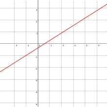
Graph of a linear function

Graph of a polynomial function, here a quadratic function.

Graph of two trigonometric functions: sine and cosine.

A real function is a real-valued function of a real variable, that is, a function whose codomain is the field of real numbers and whose domain is a set of real numbers that contains an interval. In this section, these functions are simply called functions.

The functions that are most commonly considered in mathematics and its applications have some regularity, that is they are continuous, differentiable, and even analytic. This regularity insures that these functions can be visualized by their graphs. In this section, all functions are differentiable in some interval.

Functions enjoy pointwise operations, that is, if $f$ and $g$ are functions, their sum, difference and product are functions defined by

{displaystyle {begin{aligned}(f+g)(x)&=f(x)+g(x)\(f-g)(x)&=f(x)-g(x)\(fcdot g)(x)&=f(x)cdot g(x)\end{aligned}}.}

The domains of the resulting functions are the intersection of the domains of $f$ and $g$ . The quotient of two functions is defined similarly by

{displaystyle {frac {f}{g}}(x)={frac {f(x)}{g(x)}},}

but the domain of the resulting function is obtained by removing the zeros of $g$ from the intersection of the domains of $f$ and $g$ .

The polynomial functions are defined by polynomials, and their domain is the whole set of real numbers. They include constant functions, linear functions and quadratic functions. Rational functions are quotients of two polynomial functions, and their domain is the real numbers with a finite number of them removed to avoid division by zero. The simplest rational function is the function ${displaystyle xmapsto {frac {1}{x}},}$ whose graph is a hyperbola, and whose domain is the whole real line except for 0.

The derivative of a real differentiable function is a real function. An antiderivative of a continuous real function is a real function that is differentiable in any open interval in which the original function is continuous. For example, the function ${displaystyle xmapsto {frac {1}{x}}}$ is continuous, and even differentiable, on the positive real numbers. Thus one antiderivative, which takes the value zero for $x = 1$ , is a differentiable function called the natural logarithm.

A real function $f$ is monotonic in an interval if the sign of ${displaystyle {frac {f(x)-f(y)}{x-y}}}$ does not depend of the choice of $x$ and $y$ in the interval. If the function is differentiable in the interval, it is monotonic if the sign of the derivative is constant in the interval. If a real function $f$ is monotonic in an interval $I$ , it has an inverse function, which is a real function with domain $f (I)$ and image $I$ . This is how inverse trigonometric functions are defined in terms of trigonometric functions, where the trigonometric functions are monotonic. Another example: the natural logarithm is monotonic on the positive real numbers, and its image is the whole real line; therefore it has an inverse function that is a bijection between the real numbers and the positive real numbers. This inverse is the exponential function.

Many other real functions are defined either by the implicit function theorem (the inverse function is a particular instance) or as solutions of differential equations. For example, the sine and the cosine functions are the solutions of the linear differential equation

{displaystyle y''+y=0}

such that

{displaystyle sin 0=0,quad cos 0=1,quad {frac {partial sin x}{partial x}}(0)=1,quad {frac {partial cos x}{partial x}}(0)=0.}

Vector-valued function

When the elements of the co-domain of a function are vectors the function is said to be a vector-valued function. These functions are particularly useful in applications, for example modeling physical properties. The function that associates to each point of a fluid its velocity vector is a vector-valued function.

Some vector-valued function are defined on a subset of $mathbb {R} ^{n}$ or other spaces that share geometric or topological properties similar to $mathbb {R} ^{n}$ , like manifolds. These vector-valued functions are given the name vector fields.

Function space

In mathematical analysis, and more specifically in functional analysis, a function space is a set of scalar-valued or vector-valued functions, which share a specific property and form a topological vector space. For example, the real smooth functions with a compact support (that is, they are zero outside some compact set) form a function space that is at the basis of the theory of distributions.

Function spaces play a fundamental role in advanced mathematical analysis, by allowing the use of their algebraic and topological properties for studying properties of functions. For example, all theorems of existence and uniqueness of solutions of ordinary or partial differential equations result of the study of function spaces.

Multi-valued functions

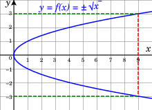
Together, the two square roots of all nonnegative real numbers form a single smooth curve.

Several methods for specifying functions of real or complex variables start from a local definition of the function at a point or on a neighbourhood of a point, and then extend by continuity the function to a much larger domain. Frequently, for a starting point $x_0,$ there are several possible starting values for the function.

For example, in defining the square root as the inverse function of the square function, for any positive real number $x_0,$ there are two choices for the value of the square root, one of which is positive and denoted ${displaystyle {sqrt {x_{0}}},}$ and another which is negative and denoted ${displaystyle -{sqrt {x_{0}}}.}$ These choices define two continuous functions, both having the nonnegative real numbers as a domain, and having either the nonnegative or the nonpositive real numbers as images. When looking at the graphs of these functions, one can see that, together, they form a single smooth curve. It is therefore often useful to consider these two square root functions as a single function that has two values for positive $x$ , one value for 0 and no value for negative $x$ .

In the preceding example, one choice, the positive square root, is more natural than the other. This is not the case in general. For example, let consider the implicit function that maps $y$ to a root $x$ of ${displaystyle x^{3}-3x-y=0}$ (see the figure on the right). For $y = 0$ one may choose either ${displaystyle 0,{sqrt {3}},{text{ or }}-{sqrt {3}}}$ for $x.$ By the implicit function theorem, each choice defines a function; for the first one, the (maximal) domain is the interval $[-2, 2]$ and the image is $[-1, 1]$ ; for the second one, the domain is $[-2, \infty)$ and the image is $[1, \infty)$ ; for the last one, the domain is $(-\infty, 2]$ and the image is $(-\infty, -1]$ . As the three graphs together form a smooth curve, and there is no reason for preferring one choice, these three functions are often considered as a single multi-valued function of $y$ that has three values for $-2 < y < 2$ , and only one value for $y \leq -2$ and $y \geq -2$ .

Usefulness of the concept of multi-valued functions is clearer when considering complex functions, typically analytic functions. The domain to which a complex function may be extended by analytic continuation generally consists of almost the whole complex plane. However, when extending the domain through two different paths, one often gets different values. For example, when extending the domain of the square root function, along a path of complex numbers with positive imaginary parts, one gets $i$ for the square root of –1; while, when extending through complex numbers with negative imaginary parts, one gets $- i$ . There are generally two ways of solving the problem. One may define a function that is not continuous along some curve, called a branch cut. Such a function is called the principal value of the function. The other way is to consider that one has a multi-valued function, which is analytic everywhere except for isolated singularities, but whose value may "jump" if one follows a closed loop around a singularity. This jump is called the monodromy.

In the foundations of mathematics and set theory

The definition of a function that is given in this article requires the concept of set, since the domain and the codomain of a function must be a set. This is not a problem in usual mathematics, as it is generally not difficult to consider only functions whose domain and codomain are sets, which are well defined, even if the domain is not explicitly defined. However, it is sometimes useful to consider more general functions.

For example, the singleton set may be considered as a function ${displaystyle xmapsto {x}.}$ Its domain would include all sets, and therefore would not be a set. In usual mathematics, one avoids this kind of problem by specifying a domain, which means that one has many singleton functions. However, when establishing foundations of mathematics, one may have to use functions whose domain, codomain or both are not specified, and some authors, often logicians, give precise definition for these weakly specified functions.^[13]

These generalized functions may be critical in the development of a formalization of the foundations of mathematics. For example, Von Neumann–Bernays–Gödel set theory, is an extension of the set theory in which the collection of all sets is a class. This theory includes the replacement axiom, which may be interpreted as "if $X$ is a set, and $F$ is a function, then $F [X]$ is a set".

In computer science

In computer programming, a function is, in general, a piece of a computer program, which implements the abstract concept of function. That is, it is a program unit that produces an output for each input. However, in many programming languages every subroutine is called a function, even when there is no output, and when the functionality consists simply of modifying some data in the computer memory.

Functional programming is the programming paradigm consisting of building programs by using only subroutines that behave like mathematical functions. For example, if_then_else is a function that takes three functions as arguments, and, depending on the result of the first function (true or false), returns the result of either the second or the third function. An important advantage of functional programming is that it makes easier program proofs, as being based on a well founded theory, the lambda calculus (see below).

Except for computer-language terminology, "function" has the usual mathematical meaning in computer science. In this area, a property of major interest is the computability of a function. For giving a precise meaning to this concept, and to the related concept of algorithm, several models of computation have been introduced, the old ones being general recursive functions, lambda calculus and Turing machine. The fundamental theorem of computability theory is that these three models of computation define the same set of computable functions, and that all the other models of computation that have ever been proposed define the same set of computable functions or a smaller one. The Church–Turing thesis is the claim that every philosophically acceptable definition of a computable function defines also the same functions.

General recursive functions are functions from integers to integers, that can be defined from the constant functions, the successor function and projection functions by mean of three operators, the composition, the primitive recursion and the minimization operators. Although defined only for functions from integers to integers, they can model any computable function, since a computation is the manipulation of finite sequences of symbols (digits of numbers, formulas, ...), and every sequence of symbols may be coded as a sequence of bits, which may also be viewed as the binary representation of an integer.

Lambda calculus is a theory that defines computable functions without using set theory, and is the theoretical background of functional programming. It consists of terms that are either variables, function definitions (λ-terms), or applications of functions to terms. Terms are manipulated through some rules, (the $α$ -equivalence, the $β$ -reduction, and the $η$ -conversion), which are the axioms of the theory and may be interpreted as rules of computation.

In its original form, lambda calculus does not include the concepts of domain and codomain of a function. Roughly speaking, they have been introduced in the theory under the name of type in typed lambda calculus. Most kinds of typed lambda calculi can define less functions than untyped lambda calculus.

^ Kaplan 1972, p. 25.

^ Gunther Schmidt( 2011) Relational Mathematics, Encyclopedia of Mathematics and its Applications, vol. 132, sect 5.1 Functions, pp. 49–60, Cambridge University Press
ISBN 978-0-521-76268-7 CUP blurb for Relational Mathematics

^ Halmos, Naive Set Theory, 1968, sect.9 ("Families")

^ Ron Larson, Bruce H. Edwards (2010), Calculus of a Single Variable, Cengage Learning, p. 19, ISBN 978-0-538-73552-0

^ T. M. Apostol (1981). Mathematical Analysis. Addison-Wesley. p. 35.

^ Lang, Serge (1971), Linear Algebra (2nd ed.), Addison-Wesley, p. 83

^ Quantities and Units - Part 2: Mathematical signs and symbols to be used in the natural sciences and technology, p. 15. ISO 80000-2 (ISO/IEC 2009-12-01)

^ Gödel 1940, p. 16; Jech 2003, p. 11; Cunningham 2016, p. 57

References

Bartle, Robert (1967). The Elements of Real Analysis. John Wiley & Sons.

Bloch, Ethan D. (2011). Proofs and Fundamentals: A First Course in Abstract Mathematics. Springer. ISBN 978-1-4419-7126-5.

Cunningham, Daniel W. (2016). Set theory: A First Course. Cambridge University Press. ISBN 978-1-107-12032-7.

Gödel, Kurt (1940). The Consistency of the Continuum Hypothesis. Princeton University Press. ISBN 978-0-691-07927-1.

Halmos, Paul R. (1970). Naive Set Theory. Springer-Verlag. ISBN 978-0-387-90092-6.

Jech, Thomas (2003). Set theory (Third Millennium ed.). Springer-Verlag. ISBN 978-3-540-44085-7.

Spivak, Michael (2008). Calculus (4th ed.). Publish or Perish. ISBN 978-0-914098-91-1.

External links

Hazewinkel, Michiel, ed. (2001) [1994], "Function", Encyclopedia of Mathematics, Springer Science+Business Media B.V. / Kluwer Academic Publishers, ISBN 978-1-55608-010-4

Weisstein, Eric W. "Function". MathWorld.

The Wolfram Functions Site gives formulae and visualizations of many mathematical functions.

NIST Digital Library of Mathematical Functions

[5] The sets X, Y are parts of data defining a function; i.e., a function is a set of ordered pairs $(x,y)$ with ${displaystyle xin X,yin Y}$ , together with the sets X, Y, such that for each $xin X$ , there is a unique $yin Y$ with $(x,y)$ in the set.

[8] This follows from the axiom of extensionality, which says two sets are the same if and only if they have the same members. Some authors drop codomain from a definition of a function, and in that definition, the notion of equality has to be handled with care; see, for example, https://math.stackexchange.com/questions/1403122/when-do-two-functions-become-equal

[14] Here "elementary" has not exactly its common sense: although most functions that are encountered in elementary courses of mathematics are elementary in this sense, some elementary functions are not elementary for the common sense, for example, those that involve roots of polynomials of high degree.

[1] The words map, mapping, transformation, correspondence, and operator are often used synonymously. Halmos 1970, p. 30.

[MacLane-2] MacLane, Saunders; Birkhoff, Garrett (1967). Algebra (First ed.). New York: Macmillan. pp. 1–13..mw-parser-output cite.citation{font-style:inherit}.mw-parser-output .citation q{quotes:"""""""'""'"}.mw-parser-output .citation .cs1-lock-free a{background:url("//upload.wikimedia.org/wikipedia/commons/thumb/6/65/Lock-green.svg/9px-Lock-green.svg.png")no-repeat;background-position:right .1em center}.mw-parser-output .citation .cs1-lock-limited a,.mw-parser-output .citation .cs1-lock-registration a{background:url("//upload.wikimedia.org/wikipedia/commons/thumb/d/d6/Lock-gray-alt-2.svg/9px-Lock-gray-alt-2.svg.png")no-repeat;background-position:right .1em center}.mw-parser-output .citation .cs1-lock-subscription a{background:url("//upload.wikimedia.org/wikipedia/commons/thumb/a/aa/Lock-red-alt-2.svg/9px-Lock-red-alt-2.svg.png")no-repeat;background-position:right .1em center}.mw-parser-output .cs1-subscription,.mw-parser-output .cs1-registration{color:#555}.mw-parser-output .cs1-subscription span,.mw-parser-output .cs1-registration span{border-bottom:1px dotted;cursor:help}.mw-parser-output .cs1-ws-icon a{background:url("//upload.wikimedia.org/wikipedia/commons/thumb/4/4c/Wikisource-logo.svg/12px-Wikisource-logo.svg.png")no-repeat;background-position:right .1em center}.mw-parser-output code.cs1-code{color:inherit;background:inherit;border:inherit;padding:inherit}.mw-parser-output .cs1-hidden-error{display:none;font-size:100%}.mw-parser-output .cs1-visible-error{font-size:100%}.mw-parser-output .cs1-maint{display:none;color:#33aa33;margin-left:0.3em}.mw-parser-output .cs1-subscription,.mw-parser-output .cs1-registration,.mw-parser-output .cs1-format{font-size:95%}.mw-parser-output .cs1-kern-left,.mw-parser-output .cs1-kern-wl-left{padding-left:0.2em}.mw-parser-output .cs1-kern-right,.mw-parser-output .cs1-kern-wl-right{padding-right:0.2em}

[FOOTNOTESpivak200839-3] Spivak 2008, p. 39.

[4] Hamilton, A. G. (1982). Numbers, sets, and axioms: the apparatus of mathematics. Cambridge University Press. p. 83. ISBN 978-0-521-24509-8.

[FOOTNOTEApostol198135-6] Apostol 1981, p. 35.

[FOOTNOTEKaplan197225-7] Kaplan 1972, p. 25.

[RM-9] Gunther Schmidt( 2011) Relational Mathematics, Encyclopedia of Mathematics and its Applications, vol. 132, sect 5.1 Functions, pp. 49–60, Cambridge University Press
ISBN 978-0-521-76268-7 CUP blurb for Relational Mathematics

[10] Halmos, Naive Set Theory, 1968, sect.9 ("Families")

[11] Ron Larson, Bruce H. Edwards (2010), Calculus of a Single Variable, Cengage Learning, p. 19, ISBN 978-0-538-73552-0

[12] T. M. Apostol (1981). Mathematical Analysis. Addison-Wesley. p. 35.

[13] Lang, Serge (1971), Linear Algebra (2nd ed.), Addison-Wesley, p. 83

[standard-15] Quantities and Units - Part 2: Mathematical signs and symbols to be used in the natural sciences and technology, p. 15. ISO 80000-2 (ISO/IEC 2009-12-01)

[16] Gödel 1940, p. 16; Jech 2003, p. 11; Cunningham 2016, p. 57

v t e Mathematical logic
General	Formal language Formation rule Formal proof Formal semantics Well-formed formula Set Element Class Classical logic Axiom Rule of inference Relation Theorem Logical consequence Type theory Symbol Syntax Theory
Systems	Formal system Deductive system Axiomatic system Hilbert style systems Natural deduction Sequent calculus
Traditional logic	Proposition Inference Argument Validity Cogency Syllogism Square of opposition Venn diagram
Propositional calculus and Boolean logic	Boolean functions Propositional calculus Propositional formula Logical connectives Truth tables Many-valued logic
Predicate logic	First-order Quantifiers Predicate Second-order Monadic predicate calculus
Naive set theory	Set Empty set Element Enumeration Extensionality Finite set Infinite set Subset Power set Countable set Uncountable set Recursive set Domain Codomain Image Map Function Relation Ordered pair
Set theory	Foundations of mathematics Zermelo–Fraenkel set theory Axiom of choice General set theory Kripke–Platek set theory Von Neumann–Bernays–Gödel set theory Morse–Kelley set theory Tarski–Grothendieck set theory
Model theory	Model Interpretation Non-standard model Finite model theory Truth value Validity
Proof theory	Formal proof Deductive system Formal system Theorem Logical consequence Rule of inference Syntax
Computability theory	Recursion Recursive set Recursively enumerable set Decision problem Church–Turing thesis Computable function Primitive recursive function

Category

Random preview

Function (mathematics)

Contents