Poisson distribution

Poisson

Probability mass function 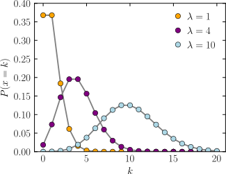The horizontal axis is the index k, the number of occurrences. λ is the expected number of occurrences, which need not be an integer. The vertical axis is the probability of k occurrences given λ. The function is defined only at integer values of k. The connecting lines are only guides for the eye.
Cumulative distribution function 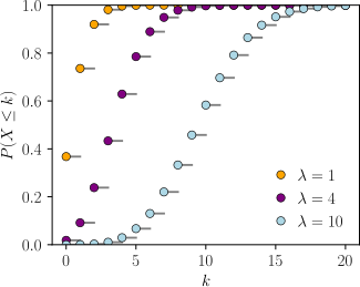The horizontal axis is the index k, the number of occurrences. The CDF is discontinuous at the integers of k and flat everywhere else because a variable that is Poisson distributed takes on only integer values.
Parameters	λ > 0 (real) — rate
Support	k∈N∪{0}{displaystyle kin mathbb {N} cup {0}}
pmf	λke−λk!{displaystyle {frac {lambda ^{k}e^{-lambda }}{k!}}}
CDF	Γ(⌊k+1⌋,λ)⌊k⌋!{displaystyle {frac {Gamma (lfloor k+1rfloor ,lambda )}{lfloor krfloor !}}}, or e−λ∑i=0⌊k⌋λii! {displaystyle e^{-lambda }sum _{i=0}^{lfloor krfloor }{frac {lambda ^{i}}{i!}} }, or Q(⌊k+1⌋,λ){displaystyle Q(lfloor k+1rfloor ,lambda )} (for k≥0{displaystyle kgeq 0}, where Γ(x,y){displaystyle Gamma (x,y)} is the upper incomplete gamma function, ⌊k⌋{displaystyle lfloor krfloor } is the floor function, and Q is the regularized gamma function)
Mean	λ{displaystyle lambda }
Median	≈⌊λ+1/3−0.02/λ⌋{displaystyle approx lfloor lambda +1/3-0.02/lambda rfloor }
Mode	⌈λ⌉−1,⌊λ⌋{displaystyle lceil lambda rceil -1,lfloor lambda rfloor }
Variance	λ{displaystyle lambda }
Skewness	λ−1/2{displaystyle lambda ^{-1/2}}
Ex. kurtosis	λ−1{displaystyle lambda ^{-1}}
Entropy	λ[1−log⁡(λ)]+e−λ∑k=0∞λklog⁡(k!)k!{displaystyle lambda [1-log(lambda )]+e^{-lambda }sum _{k=0}^{infty }{frac {lambda ^{k}log(k!)}{k!}}} (for large λ{displaystyle lambda }) 12log⁡(2πeλ)−112λ−124λ2−{displaystyle {frac {1}{2}}log(2pi elambda )-{frac {1}{12lambda }}-{frac {1}{24lambda ^{2}}}-{}} 19360λ3+O(1λ4){displaystyle qquad {frac {19}{360lambda ^{3}}}+Oleft({frac {1}{lambda ^{4}}}right)}
MGF	exp⁡(λ(et−1)){displaystyle exp(lambda (e^{t}-1))}
CF	exp⁡(λ(eit−1)){displaystyle exp(lambda (e^{it}-1))}
PGF	exp⁡(λ(z−1)){displaystyle exp(lambda (z-1))}
Fisher information	1λ{displaystyle {frac {1}{lambda }}}

In probability theory and statistics, the Poisson distribution (French pronunciation: ​[pwasɔ̃]; in English often rendered /ˈpwɑːsɒn/), named after French mathematician Siméon Denis Poisson, is a discrete probability distribution that expresses the probability of a given number of events occurring in a fixed interval of time or space if these events occur with a known constant rate and independently of the time since the last event.^[1] The Poisson distribution can also be used for the number of events in other specified intervals such as distance, area or volume.

For instance, an individual keeping track of the amount of mail they receive each day may notice that they receive an average number of 4 letters per day. If receiving any particular piece of mail does not affect the arrival times of future pieces of mail, i.e., if pieces of mail from a wide range of sources arrive independently of one another, then a reasonable assumption is that the number of pieces of mail received in a day obeys a Poisson distribution.^[2] Other examples that may follow a Poisson include the number of phone calls received by a call center per hour and the number of decay events per second from a radioactive source.

Contents

• 
  1 Basics
  
  
  
  • 
    1.1 Example
    
  
  
  • 
    1.2 Assumptions: When is the Poisson distribution an appropriate model?
    
  
  
  • 
    1.3 Probability of events for a Poisson distribution
    
    
    
    • 
      1.3.1 Examples of probability for Poisson distributions
      
    
    
    • 
      1.3.2 Once in an interval events: The special case of λ = 1 and k = 0
      
    
    
    
    
  
  
  • 
    1.4 Examples that violate the Poisson assumptions
    
  
  
  • 
    1.5 Poisson regression and negative binomial regression
    
  
  
  
  


• 
  2 History
  


• 
  3 Definition
  


• 
  4 Properties
  
  
  
  • 
    4.1 Descriptive statistics
    
  
  
  • 
    4.2 Median
    
  
  
  • 
    4.3 Higher moments
    
  
  
  • 
    4.4 Sums of Poisson-distributed random variables
    
  
  
  • 
    4.5 Other properties
    
  
  
  • 
    4.6 Poisson races
    
  
  
  
  


• 
  5 Related distributions
  


• 
  6 Occurrence
  
  
  
  • 
    6.1 Law of rare events
    
  
  
  • 
    6.2 Poisson point process
    
  
  
  • 
    6.3 Other applications in science
    
  
  
  
  


• 
  7 Generating Poisson-distributed random variables
  


• 
  8 Parameter estimation
  
  
  
  • 
    8.1 Maximum likelihood
    
  
  
  • 
    8.2 Confidence interval
    
  
  
  • 
    8.3 Bayesian inference
    
  
  
  • 
    8.4 Simultaneous estimation of multiple Poisson means
    
  
  
  
  


• 
  9 Bivariate Poisson distribution
  


• 
  10 Computer software for the Poisson distribution
  
  
  
  • 
    10.1 Poisson distribution using R
    
  
  
  • 
    10.2 Poisson distribution using Excel
    
  
  
  • 
    10.3 Poisson distribution using Mathematica
    
  
  
  
  


• 
  11 See also
  


• 
  12 Notes
  


• 
  13 Further reading
  


• 
  14 References
  

Basics

The Poisson distribution is popular for modelling the number of times an event occurs in an interval of time or space.

Example

The Poisson distribution may be useful to model events such as

• The number of meteorites greater than 1 meter diameter that strike Earth in a year


• The number of patients arriving in an emergency room between 10 and 11 pm


• The number of photons hitting a detector in a particular time interval

Assumptions: When is the Poisson distribution an appropriate model?

The Poisson distribution is an appropriate model if the following assumptions are true.

• 
  k is the number of times an event occurs in an interval and k can take values 0, 1, 2, ….


• The occurrence of one event does not affect the probability that a second event will occur. That is, events occur independently.


• The rate at which events occur is constant. The rate cannot be higher in some intervals and lower in other intervals.


• Two events cannot occur at exactly the same instant; instead, at each very small sub-interval exactly one event either occurs or does not occur.

Or

• The actual probability distribution is given by a binomial distribution and the number of trials is sufficiently bigger than the number of successes one is asking about (see Related distributions).

If these conditions are true, then k is a Poisson random variable, and the distribution of k is a Poisson distribution.

Probability of events for a Poisson distribution

An event can occur 0, 1, 2, … times in an interval. The average number of events in an interval is designated λ{displaystyle lambda } (lambda). Lambda is the event rate, also called the rate parameter. The probability of observing k events in an interval is given by the equation

P(k events in interval)=e−λλkk!{displaystyle P(k{text{ events in interval}})=e^{-lambda }{frac {lambda ^{k}}{k!}}}

where

• 
  λ{displaystyle lambda } is the average number of events per interval


• 
  e is the number 2.71828... (Euler's number) the base of the natural logarithms


• 
  k takes values 0, 1, 2, …


• 
  k! = k × (k − 1) × (k − 2) × … × 2 × 1 is the factorial of k.

This equation is the probability mass function (PMF) for a Poisson distribution.

Notice that this equation can be adapted if, instead of the average number of events λ{displaystyle lambda }, we are given a time rate r{displaystyle r} for the events to happen. Then λ=rt{displaystyle lambda =rt} (with r{displaystyle r} in units of 1/time), and

P(k events in interval t)=e−rt(rt)kk!{displaystyle P(k{text{ events in interval }}t)=e^{-rt}{frac {(rt)^{k}}{k!}}}

Examples of probability for Poisson distributions

On a particular river, overflow floods occur once every 100 years on average. Calculate the probability of k = 0, 1, 2, 3, 4, 5, or 6 overflow floods in a 100-year interval, assuming the Poisson model is appropriate.

Because the average event rate is one overflow flood per 100 years, λ = 1

P(k overflow floods in 100 years)=λke−λk!=1ke−1k!{displaystyle P(k{text{ overflow floods in 100 years}})={frac {lambda ^{k}e^{-lambda }}{k!}}={frac {1^{k}e^{-1}}{k!}}}

P(k=0 overflow floods in 100 years)=10e−10!=e−11≈0.368{displaystyle P(k=0{text{ overflow floods in 100 years}})={frac {1^{0}e^{-1}}{0!}}={frac {e^{-1}}{1}}approx 0.368}

P(k=1 overflow flood in 100 years)=11e−11!=e−11≈0.368{displaystyle P(k=1{text{ overflow flood in 100 years}})={frac {1^{1}e^{-1}}{1!}}={frac {e^{-1}}{1}}approx 0.368}

P(k=2 overflow floods in 100 years)=12e−12!=e−12≈0.184{displaystyle P(k=2{text{ overflow floods in 100 years}})={frac {1^{2}e^{-1}}{2!}}={frac {e^{-1}}{2}}approx 0.184}

The table below gives the probability for 0 to 6 overflow floods in a 100-year period.

k	P(k overflow floods in 100 years)
0	0.368
1	0.368
2	0.184
3	0.061
4	0.015
5	0.003
6	0.0005

Ugarte and colleagues report that the average number of goals in a World Cup soccer match is approximately 2.5 and the Poisson model is appropriate.^[3]

Because the average event rate is 2.5 goals per match, λ = 2.5.

P(k goals in a match)=2.5ke−2.5k!{displaystyle P(k{text{ goals in a match}})={frac {2.5^{k}e^{-2.5}}{k!}}}

P(k=0 goals in a match)=2.50e−2.50!=e−2.51≈0.082{displaystyle P(k=0{text{ goals in a match}})={frac {2.5^{0}e^{-2.5}}{0!}}={frac {e^{-2.5}}{1}}approx 0.082}

P(k=1 goal in a match)=2.51e−2.51!=2.5e−2.51≈0.205{displaystyle P(k=1{text{ goal in a match}})={frac {2.5^{1}e^{-2.5}}{1!}}={frac {2.5e^{-2.5}}{1}}approx 0.205}

P(k=2 goals in a match)=2.52e−2.52!=6.25e−2.52≈0.257{displaystyle P(k=2{text{ goals in a match}})={frac {2.5^{2}e^{-2.5}}{2!}}={frac {6.25e^{-2.5}}{2}}approx 0.257}

The table below gives the probability for 0 to 7 goals in a match.

k	P(k goals in a World Cup soccer match)
0	0.082
1	0.205
2	0.257
3	0.213
4	0.133
5	0.067
6	0.028
7	0.010

Once in an interval events: The special case of λ = 1 and k = 0

Suppose that astronomers estimate that large meteorites (above a certain size) hit the earth on average once every 100 years (λ = 1 event per 100 years), and that the number of meteorite hits follows a Poisson distribution. What is the probability of k = 0 meteorite hits in the next 100 years?

P(k=0 meteorites hit in next 100 years)=10e−10!=1e≈0.37{displaystyle P(k={text{0 meteorites hit in next 100 years}})={frac {1^{0}e^{-1}}{0!}}={frac {1}{e}}approx 0.37}

Under these assumptions, the probability that no large meteorites hit the earth in the next 100 years is roughly 0.37. The remaining 1 − 0.37 = 0.63 is the probability of 1, 2, 3, or more large meteorite hits in the next 100 years.
In an example above, an overflow flood occurred once every 100 years (λ = 1). The probability of no overflow floods in 100 years was roughly 0.37, by the same calculation.

In general, if an event occurs on average once per interval (λ = 1), and the events follow a Poisson distribution, then P(0 events in next interval) = 0.37. In addition, P(exactly one event in next interval) = 0.37, as shown in the table for overflow floods.

Examples that violate the Poisson assumptions

The number of students who arrive at the student union per minute will likely not follow a Poisson distribution, because the rate is not constant (low rate during class time, high rate between class times) and the arrivals of individual students are not independent (students tend to come in groups).

The number of magnitude 5 earthquakes per year in a country may not follow a Poisson distribution if one large earthquake increases the probability of aftershocks of similar magnitude.

Among patients admitted to the intensive care unit of a hospital, the number of days that the patients spend in the ICU is not Poisson distributed because the number of days cannot be zero. The distribution may be modeled using a Zero-truncated Poisson distribution.

Count distributions in which the number of intervals with zero events is higher than predicted by a Poisson model may be modeled using a Zero-inflated model.

Poisson regression and negative binomial regression

Poisson regression and negative binomial regression are useful for analyses where the dependent (response) variable is the count (0, 1, 2, …) of the number of events or occurrences in an interval.

History

The distribution was first introduced by Siméon Denis Poisson (1781–1840) and published, together with his probability theory, in 1837 in his work Recherches sur la probabilité des jugements en matière criminelle et en matière civile ("Research on the Probability of Judgments in Criminal and Civil Matters").^[4] The work theorized about the number of wrongful convictions in a given country by focusing on certain random variables N that count, among other things, the number of discrete occurrences (sometimes called "events" or "arrivals") that take place during a time-interval of given length. The result had been given previously by Abraham de Moivre (1711) in De Mensura Sortis seu; de Probabilitate Eventuum in Ludis a Casu Fortuito Pendentibus in Philosophical Transactions of the Royal Society, p. 219.^[5] This makes it an example of Stigler's law and it has prompted some authors to argue that the Poisson distribution should bear the name of de Moivre.^[6][7]

A practical application of this distribution was made by Ladislaus Bortkiewicz in 1898 when he was given the task of investigating the number of soldiers in the Prussian army killed accidentally by horse kicks; this experiment introduced the Poisson distribution to the field of reliability engineering.^[8]

Definition

A discrete random variable X  is said to have a Poisson distribution with parameter λ > 0, if, for k = 0, 1, 2, ..., the probability mass function of X  is given by:^[9]

f(k;λ)=Pr(X=k)=λke−λk!,{displaystyle !f(k;lambda )=Pr(X=k)={frac {lambda ^{k}e^{-lambda }}{k!}},}

where

• 
  e is Euler's number (e = 2.71828...)


• 
  k! is the factorial of k.

The positive real number λ is equal to the expected value of X and also to its variance^[10]

λ=E⁡(X)=Var⁡(X).{displaystyle lambda =operatorname {E} (X)=operatorname {Var} (X).}

The Poisson distribution can be applied to systems with a large number of possible events, each of which is rare. How many such events will occur during a fixed time interval? Under the right circumstances, this is a random number with a Poisson distribution.

The conventional definition of the Poisson distribution contains two terms that can easily overflow on computers: λ^k and k!. The fraction of λ^k to k! can also produce a rounding error that is very large compared to e^−λ, and therefore give an erroneous result. For numerical stability the Poisson probability mass function should therefore be evaluated as

f(k;λ)=exp⁡{kln⁡λ−λ−ln⁡Γ(k+1)},{displaystyle !f(k;lambda )=exp left{{kln lambda -lambda -ln Gamma (k+1)}right},}

which is mathematically equivalent but numerically stable. The natural logarithm of the Gamma function can be obtained using the lgamma function in the C (programming language) standard library (C99 version), the gammaln function in MATLAB or SciPy, or the log_gamma function in Fortran 2008 and later.

Properties

Descriptive statistics

• The expected value and variance of a Poisson-distributed random variable are both equal to λ.


• The coefficient of variation is λ−1/2{displaystyle textstyle lambda ^{-1/2}}, while the index of dispersion is 1.^[5]
  


• The mean absolute deviation about the mean is^[5]
  

E⁡|X−λ|=2exp⁡(−λ)λ⌊λ⌋+1⌊λ⌋!.{displaystyle operatorname {E} |X-lambda |=2exp(-lambda ){frac {lambda ^{lfloor lambda rfloor +1}}{lfloor lambda rfloor !}}.}

• The mode of a Poisson-distributed random variable with non-integer λ is equal to ⌊λ⌋{displaystyle scriptstyle lfloor lambda rfloor }, which is the largest integer less than or equal to λ. This is also written as floor(λ). When λ is a positive integer, the modes are λ and λ − 1.


• All of the cumulants of the Poisson distribution are equal to the expected value λ. The nth factorial moment of the Poisson distribution is λⁿ.


• The expected value of a Poisson process is sometimes decomposed into the product of intensity and exposure (or more generally expressed as the integral of an "intensity function" over time or space, sometimes described as “exposure”).^[11][12]
  

Median

Bounds for the median (ν) of the distribution are known and are sharp:^[13]

λ−ln⁡2≤ν<λ+13.{displaystyle lambda -ln 2leq nu <lambda +{frac {1}{3}}.}

Higher moments

• The higher moments m_k of the Poisson distribution about the origin are Touchard polynomials in λ:

mk=∑i=0kλi{ki},{displaystyle m_{k}=sum _{i=0}^{k}lambda ^{i}left{{begin{matrix}k\iend{matrix}}right},}

where the {braces} denote Stirling numbers of the second kind.^[14] The coefficients of the polynomials have a combinatorial meaning. In fact, when the expected value of the Poisson distribution is 1, then Dobinski's formula says that the nth moment equals the number of partitions of a set of size n.

Sums of Poisson-distributed random variables

If Xi∼Pois⁡(λi)i=1,…,n{displaystyle X_{i}sim operatorname {Pois} (lambda _{i}),i=1,dotsc ,n} are independent, and λ=∑i=1nλi{displaystyle lambda =sum _{i=1}^{n}lambda _{i}}, then Y=(∑i=1nXi)∼Pois⁡(λ){displaystyle Y=left(sum _{i=1}^{n}X_{i}right)sim operatorname {Pois} (lambda )}.^[15] A converse is Raikov's theorem, which says that if the sum of two independent random variables is Poisson-distributed, then so are each of those two independent random variables.^[16]

Other properties

• The Poisson distributions are infinitely divisible probability distributions.^[17][18]
  


• The directed Kullback–Leibler divergence of Pois(λ₀) from Pois(λ) is given by

DKL(λ∣λ0)=λ0−λ+λlog⁡λλ0.{displaystyle D_{text{KL}}(lambda mid lambda _{0})=lambda _{0}-lambda +lambda log {frac {lambda }{lambda _{0}}}.}

• Bounds for the tail probabilities of a Poisson random variable X∼Pois⁡(λ){displaystyle Xsim operatorname {Pois} (lambda )} can be derived using a Chernoff bound argument.^[19]
  

P(X≥x)≤e−λ(eλ)xxx, for x>λ{displaystyle P(Xgeq x)leq {frac {e^{-lambda }(elambda )^{x}}{x^{x}}},{text{ for }}x>lambda },

P(X≤x)≤e−λ(eλ)xxx, for x<λ.{displaystyle P(Xleq x)leq {frac {e^{-lambda }(elambda )^{x}}{x^{x}}},{text{ for }}x<lambda .}

Poisson races

Let X∼Pois⁡(λ){displaystyle Xsim operatorname {Pois} (lambda )} and Y∼Pois⁡(μ){displaystyle Ysim operatorname {Pois} (mu )} be independent random variables, with λ<μ{displaystyle lambda <mu }, then we have that

e−(μ−λ)2(λ+μ)2−e−(λ+μ)2λμ−e−(λ+μ)4λμ≤P(X−Y≥0)≤e−(μ−λ)2{displaystyle {frac {e^{-({sqrt {mu }}-{sqrt {lambda }})^{2}}}{(lambda +mu )^{2}}}-{frac {e^{-(lambda +mu )}}{2{sqrt {lambda mu }}}}-{frac {e^{-(lambda +mu )}}{4lambda mu }}leq P(X-Ygeq 0)leq e^{-({sqrt {mu }}-{sqrt {lambda }})^{2}}}

The upper bound is proved using a standard Chernoff bound.

The lower bound can be proved by noting that P(X−Y≥0∣X+Y=i){displaystyle P(X-Ygeq 0mid X+Y=i)} is the probability that Z≥i2{displaystyle Zgeq {frac {i}{2}}}, where Z∼Bin⁡(i,λλ+μ){displaystyle Zsim operatorname {Bin} left(i,{frac {lambda }{lambda +mu }}right)}, which is bounded below by 1(i+1)2e(−iD(0.5‖λλ+μ)){displaystyle {frac {1}{(i+1)^{2}}}e^{left(-iDleft(0.5|{frac {lambda }{lambda +mu }}right)right)}}, where D{displaystyle D} is relative entropy (See the entry on bounds on tails of binomial distributions for details). Further noting that X+Y∼Pois⁡(λ+μ){displaystyle X+Ysim operatorname {Pois} (lambda +mu )}, and computing a lower bound on the unconditional probability gives the result. More details can be found in the appendix of.^[20]

Related distributions

• If X1∼Pois(λ1){displaystyle X_{1}sim mathrm {Pois} (lambda _{1}),} and X2∼Pois(λ2){displaystyle X_{2}sim mathrm {Pois} (lambda _{2}),} are independent, then the difference Y=X1−X2{displaystyle Y=X_{1}-X_{2}} follows a Skellam distribution.


• If X1∼Pois(λ1){displaystyle X_{1}sim mathrm {Pois} (lambda _{1}),} and X2∼Pois(λ2){displaystyle X_{2}sim mathrm {Pois} (lambda _{2}),} are independent, then the distribution of X1{displaystyle X_{1}} conditional on X1+X2{displaystyle X_{1}+X_{2}} is a binomial distribution.

Specifically, given X1+X2=k{displaystyle X_{1}+X_{2}=k}, X1∼Binom(k,λ1/(λ1+λ2)){displaystyle !X_{1}sim mathrm {Binom} (k,lambda _{1}/(lambda _{1}+lambda _{2}))}.

More generally, if X₁, X₂,..., X_n are independent Poisson random variables with parameters λ₁, λ₂,..., λ_n then

given ∑j=1nXj=k,{displaystyle sum _{j=1}^{n}X_{j}=k,} Xi∼Binom(k,λi∑j=1nλj){displaystyle X_{i}sim mathrm {Binom} left(k,{frac {lambda _{i}}{sum _{j=1}^{n}lambda _{j}}}right)}. In fact, {Xi}∼Multinom(k,{λi∑j=1nλj}){displaystyle {X_{i}}sim mathrm {Multinom} left(k,left{{frac {lambda _{i}}{sum _{j=1}^{n}lambda _{j}}}right}right)}.

• If X∼Pois(λ){displaystyle Xsim mathrm {Pois} (lambda ),} and the distribution of Y{displaystyle Y}, conditional on X = k, is a binomial distribution, Y∣(X=k)∼Binom(k,p){displaystyle Ymid (X=k)sim mathrm {Binom} (k,p)}, then the distribution of Y follows a Poisson distribution Y∼Pois(λ⋅p){displaystyle Ysim mathrm {Pois} (lambda cdot p),}. In fact, if {Yi}{displaystyle {Y_{i}}}, conditional on X = k, follows a multinomial distribution, {Yi}∣(X=k)∼Multinom(k,pi){displaystyle {Y_{i}}mid (X=k)sim mathrm {Multinom} left(k,p_{i}right)}, then each Yi{displaystyle Y_{i}} follows an independent Poisson distribution Yi∼Pois(λ⋅pi),ρ(Yi,Yj)=0{displaystyle Y_{i}sim mathrm {Pois} (lambda cdot p_{i}),rho (Y_{i},Y_{j})=0}.


• The Poisson distribution can be derived as a limiting case to the binomial distribution as the number of trials goes to infinity and the expected number of successes remains fixed — see law of rare events below. Therefore, it can be used as an approximation of the binomial distribution if n is sufficiently large and p is sufficiently small. There is a rule of thumb stating that the Poisson distribution is a good approximation of the binomial distribution if n is at least 20 and p is smaller than or equal to 0.05, and an excellent approximation if n ≥ 100 and np ≤ 10.^[21]
  

FBinomial(k;n,p)≈FPoisson(k;λ=np){displaystyle F_{mathrm {Binomial} }(k;n,p)approx F_{mathrm {Poisson} }(k;lambda =np),}

• The Poisson distribution is a special case of the discrete compound Poisson distribution (or stuttering Poisson distribution) with only a parameter.^[22][23] The discrete compound Poisson distribution can be deduced from the limiting distribution of univariate multinomial distribution. It is also a special case of a compound Poisson distribution.


• For sufficiently large values of λ, (say λ>1000), the normal distribution with mean λ and variance λ (standard deviation λ{displaystyle {sqrt {lambda }}}) is an excellent approximation to the Poisson distribution. If λ is greater than about 10, then the normal distribution is a good approximation if an appropriate continuity correction is performed, i.e., if P(X ≤ x), where x is a non-negative integer, is replaced by P(X ≤ x + 0.5).

FPoisson(x;λ)≈Fnormal(x;μ=λ,σ2=λ){displaystyle F_{mathrm {Poisson} }(x;lambda )approx F_{mathrm {normal} }(x;mu =lambda ,sigma ^{2}=lambda ),}

• 
  Variance-stabilizing transformation: When a variable is Poisson distributed, its square root is approximately normally distributed with expected value of about λ{displaystyle {sqrt {lambda }}} and variance of about 1/4.^[24][25] Under this transformation, the convergence to normality (as λ increases) is far faster than the untransformed variable.^{[citation needed]} Other, slightly more complicated, variance stabilizing transformations are available,^[25] one of which is Anscombe transform. See Data transformation (statistics) for more general uses of transformations.


• If for every t > 0 the number of arrivals in the time interval [0, t] follows the Poisson distribution with mean λt, then the sequence of inter-arrival times are independent and identically distributed exponential random variables having mean 1/λ.^[26]
  


• The cumulative distribution functions of the Poisson and chi-squared distributions are related in the following ways:^[27]
  

FPoisson(k;λ)=1−Fχ2(2λ;2(k+1)) integer k,{displaystyle F_{text{Poisson}}(k;lambda )=1-F_{chi ^{2}}(2lambda ;2(k+1))quad quad {text{ integer }}k,}

and^[28]

Pr(X=k)=Fχ2(2λ;2(k+1))−Fχ2(2λ;2k).{displaystyle Pr(X=k)=F_{chi ^{2}}(2lambda ;2(k+1))-F_{chi ^{2}}(2lambda ;2k).}

Occurrence

Applications of the Poisson distribution can be found in many fields related to counting:^[29]

• 
  Telecommunication example: telephone calls arriving in a system.


• 
  Astronomy example: photons arriving at a telescope.


• 
  Chemistry example: the molar mass distribution of a living polymerization^[30]
  


• 
  Biology example: the number of mutations on a strand of DNA per unit length.


• 
  Management example: customers arriving at a counter or call centre.


• 
  Finance and insurance example: number of losses or claims occurring in a given period of time.


• 
  Earthquake seismology example: an asymptotic Poisson model of seismic risk for large earthquakes. (Lomnitz, 1994)^{[citation needed]}.


• 
  Radioactivity example: number of decays in a given time interval in a radioactive sample.

The Poisson distribution arises in connection with Poisson processes. It applies to various phenomena of discrete properties (that is, those that may happen 0, 1, 2, 3, ... times during a given period of time or in a given area) whenever the probability of the phenomenon happening is constant in time or space. Examples of events that may be modelled as a Poisson distribution include:

• The number of soldiers killed by horse-kicks each year in each corps in the Prussian cavalry. This example was made famous by a book of Ladislaus Josephovich Bortkiewicz (1868–1931).


• The number of yeast cells used when brewing Guinness beer. This example was made famous by William Sealy Gosset (1876–1937).^[31]
  


• The number of phone calls arriving at a call centre within a minute. This example was made famous by A.K. Erlang (1878 – 1929).


• Internet traffic.


• The number of goals in sports involving two competing teams.^[32]
  

• The number of deaths per year in a given age group.


• The number of jumps in a stock price in a given time interval.


• Under an assumption of homogeneity, the number of times a web server is accessed per minute.


• The number of mutations in a given stretch of DNA after a certain amount of radiation.


• The proportion of cells that will be infected at a given multiplicity of infection.


• The arrival of photons on a pixel circuit at a given illumination and over a given time period.


• The targeting of V-1 flying bombs on London during World War II investigated by R. D. Clarke in 1946.^[33][34]
  

Gallagher in 1976 showed that the counts of prime numbers in short intervals obey a Poisson distribution provided a certain version of an unproved conjecture of Hardy and Littlewood is true.^[35]

Law of rare events

Main article: Poisson limit theorem

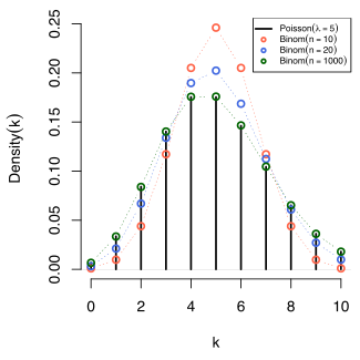
Comparison of the Poisson distribution (black lines) and the binomial distribution with n = 10 (red circles), n = 20 (blue circles), n = 1000 (green circles). All distributions have a mean of 5. The horizontal axis shows the number of events k. Notice that as n gets larger, the Poisson distribution becomes an increasingly better approximation for the binomial distribution with the same mean.

The rate of an event is related to the probability of an event occurring in some small subinterval (of time, space or otherwise). In the case of the Poisson distribution, one assumes that there exists a small enough subinterval for which the probability of an event occurring twice is "negligible". With this assumption one can derive the Poisson distribution from the Binomial one, given only the information of expected number of total events in the whole interval. Let this total number be λ{displaystyle lambda }. Divide the whole interval into n{displaystyle n} subintervals I1,…,In{displaystyle I_{1},dots ,I_{n}} of equal size, such that n{displaystyle n} > λ{displaystyle lambda } (since we are interested in only very small portions of the interval this assumption is meaningful). This means that the expected number of events in an interval Ii{displaystyle I_{i}} for each i{displaystyle i} is equal to λ/n{displaystyle lambda /n}. Now we assume that the occurrence of an event in the whole interval can be seen as a Bernoulli trial, where the ith{displaystyle i^{th}} trial corresponds to looking whether an event happens at the subinterval Ii{displaystyle I_{i}} with probability λ/n{displaystyle lambda /n}. The expected number of total events in n{displaystyle n} such trials would be λ{displaystyle lambda }, the expected number of total events in the whole interval. Hence for each subdivision of the interval we have approximated the occurrence of the event as a Bernoulli process of the form B(n,λ/n){displaystyle {textrm {B}}(n,lambda /n)}. As we have noted before we want to consider only very small subintervals. Therefore, we take the limit as n{displaystyle n} goes to infinity.
In this case the binomial distribution converges to what is known as the Poisson distribution by the Poisson limit theorem.

In several of the above examples—such as, the number of mutations in a given sequence of DNA—the events being counted are actually the outcomes of discrete trials, and would more precisely be modelled using the binomial distribution, that is

X∼B(n,p).{displaystyle Xsim {textrm {B}}(n,p).,}

In such cases n is very large and p is very small (and so the expectation np is of intermediate magnitude). Then the distribution may be approximated by the less cumbersome Poisson distribution^{[citation needed]}

X∼Pois(np).{displaystyle Xsim {textrm {Pois}}(np).,}

This approximation is sometimes known as the law of rare events,^[36] since each of the n individual Bernoulli events rarely occurs. The name may be misleading because the total count of success events in a Poisson process need not be rare if the parameter np is not small. For example, the number of telephone calls to a busy switchboard in one hour follows a Poisson distribution with the events appearing frequent to the operator, but they are rare from the point of view of the average member of the population who is very unlikely to make a call to that switchboard in that hour.

The word law is sometimes used as a synonym of probability distribution, and convergence in law means convergence in distribution. Accordingly, the Poisson distribution is sometimes called the law of small numbers because it is the probability distribution of the number of occurrences of an event that happens rarely but has very many opportunities to happen. The Law of Small Numbers is a book by Ladislaus Bortkiewicz (Bortkevitch)^[37] about the Poisson distribution, published in 1898.

Poisson point process

Main article: Poisson point process

The Poisson distribution arises as the number of points of a Poisson point process located in some finite region. More specifically, if D is some region space, for example Euclidean space R^d, for which |D|, the area, volume or, more generally, the Lebesgue measure of the region is finite, and if N(D) denotes the number of points in D, then

P(N(D)=k)=(λ|D|)ke−λ|D|k!.{displaystyle P(N(D)=k)={frac {(lambda |D|)^{k}e^{-lambda |D|}}{k!}}.}

Other applications in science

In a Poisson process, the number of observed occurrences fluctuates about its mean λ with a standard deviation σk=λ{displaystyle sigma _{k}={sqrt {lambda }}}. These fluctuations are denoted as Poisson noise or (particularly in electronics) as shot noise. See also here.

The correlation of the mean and standard deviation in counting independent discrete occurrences is useful scientifically. By monitoring how the fluctuations vary with the mean signal, one can estimate the contribution of a single occurrence, even if that contribution is too small to be detected directly. For example, the charge e on an electron can be estimated by correlating the magnitude of an electric current with its shot noise. If N electrons pass a point in a given time t on the average, the mean current is I=eN/t{displaystyle I=eN/t}; since the current fluctuations should be of the order σI=eN/t{displaystyle sigma _{I}=e{sqrt {N}}/t} (i.e., the standard deviation of the Poisson process), the charge e{displaystyle e} can be estimated from the ratio tσI2/I{displaystyle tsigma _{I}^{2}/I}.^{[citation needed]}

An everyday example is the graininess that appears as photographs are enlarged; the graininess is due to Poisson fluctuations in the number of reduced silver grains, not to the individual grains themselves. By correlating the graininess with the degree of enlargement, one can estimate the contribution of an individual grain (which is otherwise too small to be seen unaided).^{[citation needed]} Many other molecular applications of Poisson noise have been developed, e.g., estimating the number density of receptor molecules in a cell membrane.

Pr(Nt=k)=f(k;λt)=e−λt(λt)kk!.{displaystyle Pr(N_{t}=k)=f(k;lambda t)={frac {e^{-lambda t}(lambda t)^{k}}{k!}}.}

In Causal Set theory the discrete elements of spacetime follow a Poisson distribution in the volume.

Generating Poisson-distributed random variables

A simple algorithm to generate random Poisson-distributed numbers (pseudo-random number sampling) has been given by Knuth (see References below):

algorithm poisson random number (Knuth):

    init:

         Let L ← e−λ, k ← 0 and p ← 1.

    do:

         k ← k + 1.

         Generate uniform random number u in [0,1] and let p ← p × u.

    while p > L.

    return k − 1.

The complexity is linear in the returned value k, which is λ on average. There are many other algorithms to improve this. Some are given in Ahrens & Dieter, see References below. Also, for large values of λ, there may be numerical stability issues because of the term e^−λ. This could be solved by a slight change to allow λ to be added into the calculation gradually:

algorithm poisson random number (Junhao, based on Knuth):

    init:

         Let λLeft ← λ, k ← 0 and p ← 1.

    do:

         k ← k + 1.

         Generate uniform random number u in (0,1) and let p ← p × u.

         while p < 1 and λLeft > 0:

              if λLeft > STEP:

                   p ← p × eSTEP

                   λLeft ← λLeft - STEP

              else:

                   p ← p × eλLeft

                   λLeft ← 0

    while p > 1.

    return k − 1.

The choice of STEP depends on the threshold of overflow. For double precision floating point format, the threshold is near e⁷⁰⁰, so 500 shall be a safe STEP.

Other solutions for large values of λ include rejection sampling and using Gaussian approximation.

Inverse transform sampling is simple and efficient for small values of λ, and requires only one uniform random number u per sample. Cumulative probabilities are examined in turn until one exceeds u.

algorithm Poisson generator based upon the inversion by sequential search:[38]init:

         Let x ← 0, p ← e−λ, s ← p.

         Generate uniform random number u in [0,1].

    while u > s do:

         x ← x + 1.

         p ← p * λ / x.

         s ← s + p.

    return x.

"This algorithm ... requires expected time proportional to λ as λ→∞. For large λ, round-off errors proliferate, which provides us with another reason for avoiding large values of λ."^[38]

Parameter estimation

See also: Poisson regression

Maximum likelihood

Given a sample of n measured values k_i  = 0, 1, 2, ..., for i = 1, ..., n, we wish to estimate the value of the parameter λ of the Poisson population from which the sample was drawn. The maximum likelihood estimate is ^[39]

λ^MLE=1n∑i=1nki.{displaystyle {widehat {lambda }}_{mathrm {MLE} }={frac {1}{n}}sum _{i=1}^{n}k_{i}.!}

Since each observation has expectation λ so does this sample mean. Therefore, the maximum likelihood estimate is an unbiased estimator of λ. It is also an efficient estimator, i.e. its estimation variance achieves the Cramér–Rao lower bound (CRLB).^{[citation needed]} Hence it is minimum-variance unbiased. Also it can be proven that the sum (and hence the sample mean as it is a one-to-one function of the sum) is a complete and sufficient statistic for λ.

To prove sufficiency we may use the factorization theorem. Consider partitioning the probability mass function of the joint Poisson distribution for the sample into two parts: one that depends solely on the sample x{displaystyle mathbf {x} } (called h(x){displaystyle h(mathbf {x} )}) and one that depends on the parameter λ{displaystyle lambda } and the sample x{displaystyle mathbf {x} } only through the function T(x){displaystyle T(mathbf {x} )}. Then T(x){displaystyle T(mathbf {x} )} is a sufficient statistic for λ{displaystyle lambda }.

P(x)=∏i=1nλxie−λxi!=1∏i=1nxi!×λ∑i=1nxie−nλ{displaystyle P(mathbf {x} )=prod _{i=1}^{n}{frac {lambda ^{x_{i}}e^{-lambda }}{x_{i}!}}={frac {1}{prod _{i=1}^{n}x_{i}!}}times lambda ^{sum _{i=1}^{n}x_{i}}e^{-nlambda }}

Note that the first term, h(x){displaystyle h(mathbf {x} )}, depends only on x{displaystyle mathbf {x} }. The second term, g(T(x)|λ){displaystyle g(T(mathbf {x} )|lambda )}, depends on the sample only through T(x)=∑i=1nxi{displaystyle T(mathbf {x} )=sum _{i=1}^{n}x_{i}}. Thus, T(x){displaystyle T(mathbf {x} )} is sufficient.

To find the parameter λ that maximizes the probability function for the Poisson population, we can use the logarithm of the likelihood function:

ℓ(λ)=ln⁡∏i=1nf(ki∣λ)=∑i=1nln(e−λλkiki!)=−nλ+(∑i=1nki)ln⁡(λ)−∑i=1nln⁡(ki!).{displaystyle {begin{aligned}ell (lambda )&=ln prod _{i=1}^{n}f(k_{i}mid lambda )\&=sum _{i=1}^{n}ln !left({frac {e^{-lambda }lambda ^{k_{i}}}{k_{i}!}}right)\&=-nlambda +left(sum _{i=1}^{n}k_{i}right)ln(lambda )-sum _{i=1}^{n}ln(k_{i}!).end{aligned}}}

We take the derivative of ℓ{displaystyle ell } with respect to λ and compare it to zero:

ddλℓ(λ)=0⟺−n+(∑i=1nki)1λ=0.{displaystyle {frac {mathrm {d} }{mathrm {d} lambda }}ell (lambda )=0iff -n+left(sum _{i=1}^{n}k_{i}right){frac {1}{lambda }}=0.!}

Solving for λ gives a stationary point.

λ=∑i=1nkin{displaystyle lambda ={frac {sum _{i=1}^{n}k_{i}}{n}}}

So λ is the average of the k_i values. Obtaining the sign of the second derivative of L at the stationary point will determine what kind of extreme value λ is.

∂2ℓ∂λ2=−λ−2∑i=1nki{displaystyle {frac {partial ^{2}ell }{partial lambda ^{2}}}=-lambda ^{-2}sum _{i=1}^{n}k_{i}}

Evaluating the second derivative at the stationary point gives:

∂2ℓ∂λ2=−n2∑i=1nki{displaystyle {frac {partial ^{2}ell }{partial lambda ^{2}}}=-{frac {n^{2}}{sum _{i=1}^{n}k_{i}}}}

which is the negative of n times the reciprocal of the average of the k_i. This expression is negative when the average is positive. If this is satisfied, then the stationary point maximizes the probability function.

For completeness, a family of distributions is said to be complete if and only if E(g(T))=0{displaystyle E(g(T))=0} implies that Pλ(g(T)=0)=1{displaystyle P_{lambda }(g(T)=0)=1} for all λ{displaystyle lambda }. If the individual Xi{displaystyle X_{i}} are iid Po(λ){displaystyle mathrm {Po} (lambda )}, then T(x)=∑i=1nXi∼Po(nλ){displaystyle T(mathbf {x} )=sum _{i=1}^{n}X_{i}sim mathrm {Po} (nlambda )}. Knowing the distribution we want to investigate, it is easy to see that the statistic is complete.

E(g(T))=∑t=0∞g(t)(nλ)te−nλt!=0{displaystyle E(g(T))=sum _{t=0}^{infty }g(t){frac {(nlambda )^{t}e^{-nlambda }}{t!}}=0}

For this equality to hold, g(t){displaystyle g(t)} must be 0. This follows from the fact that none of the other terms will be 0 for all t{displaystyle t} in the sum and for all possible values of λ{displaystyle lambda }. Hence, E(g(T))=0{displaystyle E(g(T))=0} for all λ{displaystyle lambda } implies that Pλ(g(T)=0)=1{displaystyle P_{lambda }(g(T)=0)=1}, and the statistic has been shown to be complete.

Confidence interval

The confidence interval for the mean of a Poisson distribution can be expressed using the relationship between the cumulative distribution functions of the Poisson and chi-squared distributions. The chi-squared distribution is itself closely related to the gamma distribution, and this leads to an alternative expression. Given an observation k from a Poisson distribution with mean μ, a confidence interval for μ with confidence level 1 – α is

12χ2(α/2;2k)≤μ≤12χ2(1−α/2;2k+2),{displaystyle {tfrac {1}{2}}chi ^{2}(alpha /2;2k)leq mu leq {tfrac {1}{2}}chi ^{2}(1-alpha /2;2k+2),}

or equivalently,

F−1(α/2;k,1)≤μ≤F−1(1−α/2;k+1,1),{displaystyle F^{-1}(alpha /2;k,1)leq mu leq F^{-1}(1-alpha /2;k+1,1),}

where χ2(p;n){displaystyle chi ^{2}(p;n)} is the quantile function (corresponding to a lower tail area p) of the chi-squared distribution with n degrees of freedom and F−1(p;n,1){displaystyle F^{-1}(p;n,1)} is the quantile function of a Gamma distribution with shape parameter n and scale parameter 1.^[27][40] This interval is 'exact' in the sense that its coverage probability is never less than the nominal 1 – α.

When quantiles of the Gamma distribution are not available, an accurate approximation to this exact interval has been proposed (based on the Wilson–Hilferty transformation):^[41]

k(1−19k−zα/23k)3≤μ≤(k+1)(1−19(k+1)+zα/23k+1)3,{displaystyle kleft(1-{frac {1}{9k}}-{frac {z_{alpha /2}}{3{sqrt {k}}}}right)^{3}leq mu leq (k+1)left(1-{frac {1}{9(k+1)}}+{frac {z_{alpha /2}}{3{sqrt {k+1}}}}right)^{3},}

where zα/2{displaystyle z_{alpha /2}} denotes the standard normal deviate with upper tail area α / 2.

For application of these formulae in the same context as above (given a sample of n measured values k_i each drawn from a Poisson distribution with mean λ), one would set

k=∑i=1nki,{displaystyle k=sum _{i=1}^{n}k_{i},!}

calculate an interval for μ = nλ, and then derive the interval for λ.

Bayesian inference

In Bayesian inference, the conjugate prior for the rate parameter λ of the Poisson distribution is the gamma distribution.^[42] Let

λ∼Gamma(α,β){displaystyle lambda sim mathrm {Gamma} (alpha ,beta )!}

denote that λ is distributed according to the gamma density g parameterized in terms of a shape parameter α and an inverse scale parameter β:

g(λ∣α,β)=βαΓ(α)λα−1e−βλ for λ>0.{displaystyle g(lambda mid alpha ,beta )={frac {beta ^{alpha }}{Gamma (alpha )}};lambda ^{alpha -1};e^{-beta ,lambda }qquad {text{ for }}lambda >0,!.}

Then, given the same sample of n measured values k_ias before, and a prior of Gamma(α, β), the posterior distribution is

λ∼Gamma(α+∑i=1nki,β+n).{displaystyle lambda sim mathrm {Gamma} left(alpha +sum _{i=1}^{n}k_{i},beta +nright).!}

The posterior mean E[λ] approaches the maximum likelihood estimate λ^MLE{displaystyle {widehat {lambda }}_{mathrm {MLE} }} in the limit as α→0, β→0{displaystyle alpha to 0, beta to 0}, which follows immediately from the general expression of the mean of the gamma distribution.

The posterior predictive distribution for a single additional observation is a negative binomial distribution,^[43] sometimes called a Gamma–Poisson distribution.

Simultaneous estimation of multiple Poisson means

Suppose X1,X2,…,Xp{displaystyle X_{1},X_{2},dots ,X_{p}} is a set of independent random variables from a set of p{displaystyle p} Poisson distributions, each with a parameter λi{displaystyle lambda _{i}}, i=1,…,p{displaystyle i=1,dots ,p}, and we would like to estimate these parameters. Then, Clevenson and Zidek show that under the normalized squared error loss L(λ,λ^)=∑i=1pλi−1(λ^i−λi)2{displaystyle L(lambda ,{hat {lambda }})=sum _{i=1}^{p}lambda _{i}^{-1}({hat {lambda }}_{i}-lambda _{i})^{2}}, when p>1{displaystyle p>1}, then, similar as in Stein's famous example for the Normal means, the MLE estimator λ^i=Xi{displaystyle {hat {lambda }}_{i}=X_{i}} is inadmissible.^[44]

In this case, a family of minimax estimators is given for any 0<c≤2(p−1){displaystyle 0<cleq 2(p-1)} and b≥(p−2+p−1){displaystyle bgeq (p-2+p^{-1})} as^[45]

λ^i=(1−cb+∑i=1pXi)Xi,i=1,…,p.{displaystyle {hat {lambda }}_{i}=left(1-{frac {c}{b+sum _{i=1}^{p}X_{i}}}right)X_{i},qquad i=1,dots ,p.}

Bivariate Poisson distribution

This distribution has been extended to the bivariate case.^[46] The generating function for this distribution is

g(u,v)=exp⁡[(θ1−θ12)(u−1)+(θ2−θ12)(v−1)+θ12(uv−1)]{displaystyle g(u,v)=exp[(theta _{1}-theta _{12})(u-1)+(theta _{2}-theta _{12})(v-1)+theta _{12}(uv-1)]}

with

θ1,θ2>θ12>0{displaystyle theta _{1},theta _{2}>theta _{12}>0,}

The marginal distributions are Poisson(θ₁) and Poisson(θ₂) and the correlation coefficient is limited to the range

0≤ρ≤min{θ1θ2,θ2θ1}{displaystyle 0leq rho leq min left{{frac {theta _{1}}{theta _{2}}},{frac {theta _{2}}{theta _{1}}}right}}

A simple way to generate a bivariate Poisson distribution X1,X2{displaystyle X_{1},X_{2}} is to take three independent Poisson distributions Y1,Y2,Y3{displaystyle Y_{1},Y_{2},Y_{3}} with means λ1,λ2,λ3{displaystyle lambda _{1},lambda _{2},lambda _{3}} and then set X1=Y1+Y3,X2=Y2+Y3{displaystyle X_{1}=Y_{1}+Y_{3},X_{2}=Y_{2}+Y_{3}}. The probability function of the bivariate Poisson distribution is

Pr(X1=k1,X2=k2)=exp⁡(−λ1−λ2−λ3)λ1k1k1!λ2k2k2!∑k=0min(k1,k2)(k1k)(k2k)k!(λ3λ1λ2)k{displaystyle {begin{aligned}&Pr(X_{1}=k_{1},X_{2}=k_{2})\={}&exp left(-lambda _{1}-lambda _{2}-lambda _{3}right){frac {lambda _{1}^{k_{1}}}{k_{1}!}}{frac {lambda _{2}^{k_{2}}}{k_{2}!}}sum _{k=0}^{min(k_{1},k_{2})}{binom {k_{1}}{k}}{binom {k_{2}}{k}}k!left({frac {lambda _{3}}{lambda _{1}lambda _{2}}}right)^{k}end{aligned}}}

Computer software for the Poisson distribution

Poisson distribution using R

The R function dpois(x, lambda) calculates the probability that there are x events in an interval, where the argument "lambda" is the average number of events per interval.

For example,

dpois(x=0, lambda=1) = 0.3678794

dpois(x=1, lambda=2.5) = 0.2052125

The following R code creates a graph of the Poisson distribution from x= 0 to 8, with lambda=2.5.

x=0:8

px = dpois(x, lambda=2.5)

plot(x, px, type="h", xlab="Number of events k", ylab="Probability of k events", ylim=c(0,0.5), pty="s", main="Poisson distribution n Probability of events for lambda = 2.5")

Poisson distribution using Excel

The Excel function POISSON( x, mean, cumulative ) calculates the probability of x events where mean is lambda, the average number of events per interval. The argument cumulative specifies the cumulative distribution.

For example,

=POISSON(0, 1, FALSE) = 0.3678794

=POISSON(1, 2.5, FALSE) = 0.2052125

Poisson distribution using Mathematica

Mathematica supports the univariate Poisson distribution as PoissonDistribution[λ{displaystyle lambda }],^[47] and the bivariate Poisson distribution as MultivariatePoissonDistribution[θ12{displaystyle theta _{12}},{ θ1−θ12{displaystyle theta _{1}-theta _{12}}, θ2−θ12{displaystyle theta _{2}-theta _{12}}}],^[48] including computation of probabilities and expectation, sampling, parameter estimation and hypothesis testing.

See also

• Compound Poisson distribution


• Conway–Maxwell–Poisson distribution


• Erlang distribution


• Hermite distribution


• Index of dispersion


• Negative binomial distribution


• Poisson clumping


• Poisson point process


• Poisson regression


• Poisson sampling


• Poisson wavelet


• Queueing theory


• Renewal theory


• Robbins lemma


• 
  Skellam distribution (distribution of the difference of two Poisson distributed variates)


• Tweedie distribution


• Zero-inflated model


• Zero-truncated Poisson distribution

Notes

1. 
   ^ Frank A. Haight (1967). Handbook of the Poisson Distribution. New York: John Wiley & Sons..mw-parser-output cite.citation{font-style:inherit}.mw-parser-output q{quotes:"""""""'""'"}.mw-parser-output code.cs1-code{color:inherit;background:inherit;border:inherit;padding:inherit}.mw-parser-output .cs1-lock-free a{background:url("//upload.wikimedia.org/wikipedia/commons/thumb/6/65/Lock-green.svg/9px-Lock-green.svg.png")no-repeat;background-position:right .1em center}.mw-parser-output .cs1-lock-limited a,.mw-parser-output .cs1-lock-registration a{background:url("//upload.wikimedia.org/wikipedia/commons/thumb/d/d6/Lock-gray-alt-2.svg/9px-Lock-gray-alt-2.svg.png")no-repeat;background-position:right .1em center}.mw-parser-output .cs1-lock-subscription a{background:url("//upload.wikimedia.org/wikipedia/commons/thumb/a/aa/Lock-red-alt-2.svg/9px-Lock-red-alt-2.svg.png")no-repeat;background-position:right .1em center}.mw-parser-output .cs1-subscription,.mw-parser-output .cs1-registration{color:#555}.mw-parser-output .cs1-subscription span,.mw-parser-output .cs1-registration span{border-bottom:1px dotted;cursor:help}.mw-parser-output .cs1-hidden-error{display:none;font-size:100%}.mw-parser-output .cs1-visible-error{font-size:100%}.mw-parser-output .cs1-subscription,.mw-parser-output .cs1-registration,.mw-parser-output .cs1-format{font-size:95%}.mw-parser-output .cs1-kern-left,.mw-parser-output .cs1-kern-wl-left{padding-left:0.2em}.mw-parser-output .cs1-kern-right,.mw-parser-output .cs1-kern-wl-right{padding-right:0.2em}
   


2. 
   ^ "Statistics | The Poisson Distribution". Umass.edu. 2007-08-24. Retrieved 2014-04-18.
   


3. 
   ^ Ugarte, MD; Militino, AF; Arnholt, AT (2016), Probability and Statistics with R (Second ed.), CRC Press, ISBN 978-1-4665-0439-4
   


4. 
   ^ S.D. Poisson, Probabilité des jugements en matière criminelle et en matière civile, précédées des règles générales du calcul des probabilitiés (Paris, France: Bachelier, 1837), page 206.
   


5. 
   ^ ^abc Johnson, N.L., Kotz, S., Kemp, A.W. (1993) Univariate Discrete distributions (2nd edition). Wiley.
   ISBN 0-471-54897-9, p157
   


6. 
   ^ Stigler, Stephen M. (1982). "Poisson on the poisson distribution". Statistics & Probability Letters. 1: 33–35. doi:10.1016/0167-7152(82)90010-4.
   


7. 
   ^ Hald, A.; de Moivre, Abraham; McClintock, Bruce (1984). "A. de Moivre: 'De Mensura Sortis' or 'On the Measurement of Chance'". International Statistical Review / Revue Internationale de Statistique. 52 (3): 229–262. doi:10.2307/1403045. JSTOR 1403045.
   


8. 
   ^ Ladislaus von Bortkiewicz, Das Gesetz der kleinen Zahlen [The law of small numbers] (Leipzig, Germany: B.G. Teubner, 1898). On page 1, Bortkiewicz presents the Poisson distribution. On pages 23–25, Bortkiewicz presents his famous analysis of "4. Beispiel: Die durch Schlag eines Pferdes im preussischen Heere Getöteten." (4. Example: Those killed in the Prussian army by a horse's kick.).
   


9. 
   ^ Probability and Stochastic Processes: A Friendly Introduction for Electrical and Computer Engineers, Roy D. Yates, David Goodman, page 60.
   


10. 
    ^ For the proof, see :
    Proof wiki: expectation and Proof wiki: variance
    


11. 
    ^ Some Poisson models, Vose Software, retrieved 2016-01-18
    


12. 
    ^ Helske, Jouni (2015-06-25), KFAS: Exponential family state space models in R (PDF), Comprehensive R Archive Network, retrieved 2016-01-18
    


13. 
    ^ Choi KP (1994) On the medians of Gamma distributions and an equation of Ramanujan. Proc Amer Math Soc 121 (1) 245–251
    


14. 
    ^ Riordan, John (1937). "Moment recurrence relations for binomial, Poisson and hypergeometric frequency distributions". Annals of Mathematical Statistics. 8 (2): 103–111. doi:10.1214/aoms/1177732430. Also see Haight (1967), p. 6.
    


15. 
    ^ E. L. Lehmann (1986). Testing Statistical Hypotheses (second ed.). New York: Springer Verlag. ISBN 978-0-387-94919-2. page 65.
    


16. 
    ^ Raikov, D. (1937). On the decomposition of Poisson laws. Comptes Rendus de l'Académie des Sciences de l'URSS, 14, 9–11. (The proof is also given in von Mises, Richard (1964). Mathematical Theory of Probability and Statistics. New York: Academic Press.)
    


17. 
    ^ Laha, R. G. & Rohatgi, V. K. (1979-05-01). Probability Theory. New York: John Wiley & Sons. p. 233. ISBN 978-0-471-03262-5.
    


18. 
    ^ Johnson, N.L., Kotz, S., Kemp, A.W. (1993) Univariate Discrete distributions (2nd edition). Wiley.
    ISBN 0-471-54897-9, p159
    


19. 
    ^ Michael Mitzenmacher & Eli Upfal (2005-01-31). Probability and Computing: Randomized Algorithms and Probabilistic Analysis. Cambridge University Press. p. 97. ISBN 978-0521835404.
    


20. 
    ^ "Optimal Haplotype Assembly from High-Throughput Mate-Pair Reads, published in ISIT 2015"
    


21. 
    ^ NIST/SEMATECH, '6.3.3.1. Counts Control Charts', e-Handbook of Statistical Methods, accessed 25 October 2006
    


22. 
    ^ Huiming, Zhang; Yunxiao Liu; Bo Li (2014). "Notes on discrete compound Poisson model with applications to risk theory". Insurance: Mathematics and Economics. 59: 325–336. doi:10.1016/j.insmatheco.2014.09.012.
    


23. 
    ^ Huiming, Zhang; Bo Li (2016). "Characterizations of discrete compound Poisson distributions". Communications in Statistics - Theory and Methods. 45 (22): 6789–6802. doi:10.1080/03610926.2014.901375.
    


24. 
    ^ McCullagh, Peter; Nelder, John (1989). Generalized Linear Models. London: Chapman and Hall. ISBN 978-0-412-31760-6. page 196 gives the approximation and higher order terms.
    


25. 
    ^ ^ab Johnson, N.L., Kotz, S., Kemp, A.W. (1993) Univariate Discrete distributions (2nd edition). Wiley.
    ISBN 0-471-54897-9, p163
    


26. 
    ^ S. M. Ross (2007). Introduction to Probability Models (ninth ed.). Boston: Academic Press. ISBN 978-0-12-598062-3. pp. 307–308.
    


27. 
    ^ ^ab Johnson, N.L., Kotz, S., Kemp, A.W. (1993) Univariate Discrete distributions (2nd edition). Wiley.
    ISBN 0-471-54897-9, p171
    


28. 
    ^ Johnson, N.L., Kotz, S., Kemp, A.W. (1993) Univariate Discrete distributions (2nd edition). Wiley.
    ISBN 0-471-54897-9, p153
    


29. 
    ^ "The Poisson Process as a Model for a Diversity of Behavioural Phenomena"
    


30. 
    ^ Paul J. Flory (1940). "Molecular Size Distribution in Ethylene Oxide Polymers". Journal of the American Chemical Society. 62 (6): 1561–1565. doi:10.1021/ja01863a066.
    


31. 
    ^ Philip J. Boland (1984). "A Biographical Glimpse of William Sealy Gosset". The American Statistician. 38 (3): 179–183. doi:10.1080/00031305.1984.10483195.
    


32. 
    ^
    Dave Hornby. "Football Prediction Model: Poisson Distribution". calculate the probability of outcomes for a football match, which in turn can be turned into odds that we can use to identify value in the market.
    


33. 
    ^ Clarke, R. D. (1946). "An application of the Poisson distribution". Journal of the Institute of Actuaries. 72: 481.
    


34. 
    ^
    Aatish Bhatia (2012-12-21). "What does randomness look like?". Wired. Within a large area of London, the bombs weren’t being targeted. They rained down at random in a devastating, city-wide game of Russian roulette.
    


35. 
    ^ P.X., Gallagher (1976). "On the distribution of primes in short intervals". Mathematika. 23: 4–9. doi:10.1112/s0025579300016442.
    


36. 
    ^ A. Colin Cameron; Pravin K. Trivedi (1998). Regression Analysis of Count Data. ISBN 9780521635677. Retrieved 2013-01-30. (p.5) The law of rare events states that the total number of events will follow, approximately, the Poisson distribution if an event may occur in any of a large number of trials but the probability of occurrence in any given trial is small.
    


37. 
    ^ Edgeworth, F. Y. (1913). "On the use of the theory of probabilities in statistics relating to society". Journal of the Royal Statistical Society. 76 (2): 165–193. doi:10.2307/2340091. JSTOR 10.2307/2340091.
    


38. 
    ^ ^ab Devroye, Luc (1986). "Discrete Univariate Distributions" (PDF). Non-Uniform Random Variate Generation. New York: Springer-Verlag. p. 505.
    


39. 
    ^ Paszek, Ewa. "Maximum Likelihood Estimation – Examples".
    


40. 
    ^
    Garwood, F. (1936). "Fiducial Limits for the Poisson Distribution". Biometrika. 28 (3/4): 437–442. doi:10.1093/biomet/28.3-4.437.
    


41. 
    ^ Breslow, NE; Day, NE (1987). Statistical Methods in Cancer Research: Volume 2—The Design and Analysis of Cohort Studies. Paris: International Agency for Research on Cancer. ISBN 978-92-832-0182-3.
    


42. 
    ^ Fink, Daniel (1997). A Compendium of Conjugate Priors.
    


43. 
    ^ Gelman; et al. (2005). Bayesian Data Analysis (2nd ed.). p. 60.
    


44. 
    ^ Clevenson, M. L.; Zidek, J. V. (1975). "Simultaneous Estimation of the Means of Independent Poisson Laws". Journal of the American Statistical Association. 70 (351a): 698–705. doi:10.1080/01621459.1975.10482497.
    


45. 
    ^ Berger, J. O. (1985). Statistical Decision Theory and Bayesian Analysis (2nd ed.). Springer.
    


46. 
    ^ Loukas, S.; Kemp, C. D. (1986). "The Index of Dispersion Test for the Bivariate Poisson Distribution". Biometrics. 42 (4): 941–948. doi:10.2307/2530708. JSTOR 2530708.
    


47. 
    ^ "Wolfram Language: PoissonDistribution reference page". wolfram.com. Retrieved 2016-04-08.
    


48. 
    ^ "Wolfram Language: MultivariatePoissonDistribution reference page". wolfram.com. Retrieved 2016-04-08.
    

Further reading

• 
  Shanmugam, Ramalingam (2013). "Informatics about fear to report rapes using bumped-up Poisson model". American Journal of Biostatistics. 3 (1): 17–29. doi:10.3844/amjbsp.2013.17.29.
  

References

• 
  Joachim H. Ahrens; Ulrich Dieter (1974). "Computer Methods for Sampling from Gamma, Beta, Poisson and Binomial Distributions". Computing. 12 (3): 223–246. doi:10.1007/BF02293108.
  


• 
  Joachim H. Ahrens; Ulrich Dieter (1982). "Computer Generation of Poisson Deviates". ACM Transactions on Mathematical Software. 8 (2): 163–179. doi:10.1145/355993.355997.
  


• 
  Ronald J. Evans; J. Boersma; N. M. Blachman; A. A. Jagers (1988). "The Entropy of a Poisson Distribution: Problem 87-6". SIAM Review. 30 (2): 314–317. doi:10.1137/1030059.
  


• 
  Donald E. Knuth (1969). Seminumerical Algorithms. The Art of Computer Programming, Volume 2. Addison Wesley.
  

v t e Probability distributions
List
Discrete univariate with finite support	Benford Bernoulli beta-binomial binomial categorical hypergeometric Poisson binomial Rademacher soliton discrete uniform Zipf Zipf–Mandelbrot
Discrete univariate with infinite support	beta negative binomial Borel Conway–Maxwell–Poisson discrete phase-type Delaporte extended negative binomial Gauss–Kuzmin geometric logarithmic negative binomial parabolic fractal Poisson Skellam Yule–Simon zeta
Continuous univariate supported on a bounded interval	arcsine ARGUS Balding–Nichols Bates beta beta rectangular Irwin–Hall Kumaraswamy logit-normal noncentral beta raised cosine reciprocal triangular U-quadratic uniform Wigner semicircle
Continuous univariate supported on a semi-infinite interval	Benini Benktander 1st kind Benktander 2nd kind beta prime Burr chi-squared chi Dagum Davis exponential-logarithmic Erlang exponential F folded normal Flory–Schulz Fréchet gamma gamma/Gompertz generalized inverse Gaussian Gompertz half-logistic half-normal Hotelling's T-squared hyper-Erlang hyperexponential hypoexponential inverse chi-squared scaled inverse chi-squared inverse Gaussian inverse gamma Kolmogorov Lévy log-Cauchy log-Laplace log-logistic log-normal Lomax matrix-exponential Maxwell–Boltzmann Maxwell–Jüttner Mittag-Leffler Nakagami noncentral chi-squared Pareto phase-type poly-Weibull Rayleigh relativistic Breit–Wigner Rice shifted Gompertz truncated normal type-2 Gumbel Weibull Discrete Weibull Wilks's lambda
Continuous univariate supported on the whole real line	Cauchy exponential power Fisher's z Gaussian q generalized normal generalized hyperbolic geometric stable Gumbel Holtsmark hyperbolic secant Johnson's SU Landau Laplace asymmetric Laplace logistic noncentral t normal (Gaussian) normal-inverse Gaussian skew normal slash stable Student's t type-1 Gumbel Tracy–Widom variance-gamma Voigt
Continuous univariate with support whose type varies	generalized extreme value generalized Pareto Marchenko–Pastur q-exponential q-Gaussian q-Weibull shifted log-logistic Tukey lambda
Mixed continuous-discrete univariate	rectified Gaussian
Multivariate (joint)	.mw-parser-output .nobold{font-weight:normal} Discrete Ewens multinomial Dirichlet-multinomial negative multinomial Continuous Dirichlet generalized Dirichlet multivariate Laplace multivariate normal multivariate stable multivariate t normal-inverse-gamma normal-gamma Matrix-valued inverse matrix gamma inverse-Wishart matrix normal matrix t matrix gamma normal-inverse-Wishart normal-Wishart Wishart
Directional	Univariate (circular) directional Circular uniform univariate von Mises wrapped normal wrapped Cauchy wrapped exponential wrapped asymmetric Laplace wrapped Lévy Bivariate (spherical) Kent Bivariate (toroidal) bivariate von Mises Multivariate von Mises–Fisher Bingham
Degenerate and singular	Degenerate Dirac delta function Singular Cantor
Families	Circular compound Poisson elliptical exponential natural exponential location–scale maximum entropy mixture Pearson Tweedie wrapped

Authority control	GND: 4253010-6 LCCN: sh85103956 NDL: 00569122

This page is only for reference, If you need detailed information, please check here