 Mixing
Dose–response relationship
Semi-log plots of the hypothetical response to agonist, log concentration on the x-axis, in combination with different antagonist concentrations. The parameters of the curves, and how the antagonist changes them, gives useful information about the agonist's pharmacological profile. This curve is similar but distinct from that, which is generated with the ligand-bound receptor concentration on the y-axis.
The dose–response relationship, or exposure–response relationship, describes the magnitude of the response of an organism, as a function of exposure (or doses) to a stimulus or stressor (usually a chemical) after a certain exposure time.[1] Dose-response relationships can be described by dose-response curves. This is explained further in the following sections. A stimulus response function or stimulus response curve is defined more broadly as the response from any type of stimulus, not limited to chemicals.
Contents
1 Motivation for Studying Dose-Response Relationships
1.1 Example Stimuli and Responses
2 Analysis and Creation of Dose Response Curves
2.1 Construction of Dose-Response Curves
2.1.1 Hill Equation
2.2 Units of Dose-Response Relationship
3 Limitations
3.1 Problems with linear model
3.2 Factors affecting Dose-Response Relationships
4 Schild Analysis
5 See also
6 References
7 External links
Motivation for Studying Dose-Response Relationships
Studying dose response, and developing dose–response models, is central to determining "safe", "hazardous" and (where relevant) beneficial levels and dosages for drugs, pollutants, foods, and other substances to which humans or other organisms are exposed. These conclusions are often the basis for public policy. The U.S. Environmental Protection Agency has developed extensive guidance and reports on dose-response modeling and assessment, as well as software.[2] The U.S. Food and Drug Administration also has guidance to elucidate dose-response relationships[3] during drug development. Dose response relationships may be used in individuals or in populations. The adage The dose makes the poison reflects how a small amount of a toxin has no significant effect, while a large amount may be fatal. This reflects how dose-response relationships can be used in individuals. In populations, dose-response relationships can describe the way groups of people or organisms are affected at different levels of exposure. Dose response relationships modelled by dose response curves are used extensively in pharmacology and drug development. In particular, the shape of a drug's dose-response curve (quantified by EC50, nH and ymax parameters) reflects the biological activity and strength of the drug.
Example Stimuli and Responses
Some example measures for dose-response relationships are shown in the tables below. Each sensory stimulus corresponds with a particular sensory receptor, for instance the nicotinic acetylcholine receptor for nicotine, or the mechanoreceptor for mechanical pressure. However, stimuli (such as temperatures or radiation) may also affect physiological processes beyond sensation (and even give the measurable response of death).
| Example Stimulus | Sensory Receptor | |
|---|---|---|
Drug/Toxin dose | Agonist (e.g. nicotine, isoprenaline) | Biochemical receptors |
Antagonist (e.g. ketamine, propranolol) | ||
Allosteric modulator (e.g. Benzodiazepine) | ||
Temperature | Temperature receptors | |
| Sound levels | Hair cells | |
| Illumination/Light intensity | Photoreceptors | |
| Mechanical pressure | Mechanoreceptors | |
| Pathogen dose | n/a | |
Radiation intensity | n/a | |
| System Level | Example Response | Response Data type | |
|---|---|---|---|
Population | Epidemiology
| Death[4], loss of consciousness | Count[4]/Proportion |
Organism (Whole animal) | Severity of lesion[4] | Descriptive[4] | |
Organ | Blood pressure[4] | Continuous[4] | |
Tissue | ATP production | - | |
Cell | ATP production | - | |
Analysis and Creation of Dose Response Curves
Construction of Dose-Response Curves
A dose–response curve is a coordinate graph relating the magnitude of a stimulus to the response of the receptor. A number of effects (or endpoints) can be studied. The measured dose is generally plotted on the X axis and the response is plotted on the Y axis. In some cases, it is the logarithm of the dose that is plotted on the X axis, and in such cases the curve is typically sigmoidal, with the steepest portion in the middle. Biologically based models using dose are preferred over the use of log(dose) because the latter can visually imply a threshold dose when in fact there is none.[citation needed]
Statistical analysis of dose-response curves may be performed by regression methods such as the probit model or logit model, or other methods such as the Spearman-Karber method.[5] Empirical models based on nonlinear regression are usually preferred over the use of some transformation of the data that linearizes the dose-response relationship.[6]
Hill Equation
Dose–response curves are generally sigmoidal and monophasic and can be fit to a classical Hill equation. The Hill equation is logistic equation with respect to the logarithm of the dose and is similar to a logit model. A generalized model for multiphasic cases has also been suggested.[7]
The Hill equation is the following formula, where E{displaystyle E}
![{displaystyle {ce {[A]}}}](https://wikimedia.org/api/rest_v1/media/math/render/svg/881146b6653b24508d87e34a81c84832f1d5ffea)


EEmax=11+(EC50[A])n{displaystyle {frac {E}{E_{mathrm {max} }}}={frac {1}{1+left({frac {mathrm {EC} _{50}}{[A]}}right)^{n}}}}[8]
The parameters of the dose response curve reflect measures of potency (such as EC50, IC50, ED50, etc.) and measures of efficacy (such as tissue, cell or population response).
A commonly used dose-response curve is the EC50 curve, the half maximal effective concentration, where the EC50 point is defined as the inflection point of the curve.
Dose response curves are typically fitted to the Hill equation.
The first point along the graph where a response above zero (or above the control response) is reached is usually referred to as a threshold-dose. For most beneficial or recreational drugs, the desired effects are found at doses slightly greater than the threshold dose. At higher doses, undesired side effects appear and grow stronger as the dose increases. The more potent a particular substance is, the steeper this curve will be. In quantitative situations, the Y-axis often is designated by percentages, which refer to the percentage of exposed individuals registering a standard response (which may be death, as in LD50). Such a curve is referred to as a quantal dose-response curve, distinguishing it from a graded dose-response curve, where response is continuous (either measured, or by judgment).
The Hill equation can be used to describe dose-response relationships, for example ion channel-open-probability vs. ligand concentration.[9]
Units of Dose-Response Relationship
Dose is usually in milligrams, micrograms, or grams per kilogram of body-weight for oral exposures or milligrams per cubic meter of ambient air for inhalation exposures. Other dose units include moles per body-weight, moles per animal, and for dermal exposure, moles per square centimeter.
Limitations
Problems with linear model
The concept of linear dose-response relationship, thresholds, and all-or-nothing responses may not apply to non-linear situations. A threshold model or linear no-threshold model may be more appropriate, depending on the circumstances.
A recent critique of these models as they apply to endocrine disruptors argues for a substantial revision of testing and toxicological models at low doses because of observed non-monotonicity, i.e. U-shaped dose/response curves.[10]
Factors affecting Dose-Response Relationships
Dose–response relationships generally depend on the exposure time and exposure route (e.g., inhalation, dietary intake); quantifying the response after a different exposure time or for a different route leads to a different relationship and possibly different conclusions on the effects of the stressor under consideration. This limitation is caused by the complexity of biological systems and the often unknown biological processes operating between the external exposure and the adverse cellular or tissue response.
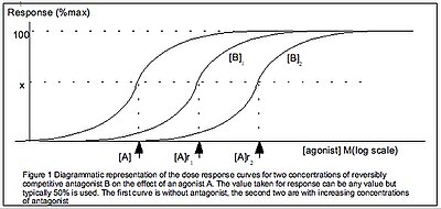
Schild Analysis
Schild analysis may also provide insights into the effect of drugs.
See also
- Arndt-Schulz rule
- Ceiling effect (pharmacology)
- Certain safety factor
- Hormesis
- IC50
- Pharmacodynamics
- Schild regression
- Spatial epidemiology
- Weber–Fechner law
- Dose fractionation
- The dose makes the poison
- Hill equation (biochemistry)
References
^ Crump, KS; Hoel, DG; Langley, CH; Peto, R (1976). "Fundamental carcinogenic processes and their implications for low dose risk assessment". Cancer Research. 36 (9 Part1): 2973–9. PMID 975067..mw-parser-output cite.citation{font-style:inherit}.mw-parser-output .citation q{quotes:"""""""'""'"}.mw-parser-output .citation .cs1-lock-free a{background:url("//upload.wikimedia.org/wikipedia/commons/thumb/6/65/Lock-green.svg/9px-Lock-green.svg.png")no-repeat;background-position:right .1em center}.mw-parser-output .citation .cs1-lock-limited a,.mw-parser-output .citation .cs1-lock-registration a{background:url("//upload.wikimedia.org/wikipedia/commons/thumb/d/d6/Lock-gray-alt-2.svg/9px-Lock-gray-alt-2.svg.png")no-repeat;background-position:right .1em center}.mw-parser-output .citation .cs1-lock-subscription a{background:url("//upload.wikimedia.org/wikipedia/commons/thumb/a/aa/Lock-red-alt-2.svg/9px-Lock-red-alt-2.svg.png")no-repeat;background-position:right .1em center}.mw-parser-output .cs1-subscription,.mw-parser-output .cs1-registration{color:#555}.mw-parser-output .cs1-subscription span,.mw-parser-output .cs1-registration span{border-bottom:1px dotted;cursor:help}.mw-parser-output .cs1-ws-icon a{background:url("//upload.wikimedia.org/wikipedia/commons/thumb/4/4c/Wikisource-logo.svg/12px-Wikisource-logo.svg.png")no-repeat;background-position:right .1em center}.mw-parser-output code.cs1-code{color:inherit;background:inherit;border:inherit;padding:inherit}.mw-parser-output .cs1-hidden-error{display:none;font-size:100%}.mw-parser-output .cs1-visible-error{font-size:100%}.mw-parser-output .cs1-maint{display:none;color:#33aa33;margin-left:0.3em}.mw-parser-output .cs1-subscription,.mw-parser-output .cs1-registration,.mw-parser-output .cs1-format{font-size:95%}.mw-parser-output .cs1-kern-left,.mw-parser-output .cs1-kern-wl-left{padding-left:0.2em}.mw-parser-output .cs1-kern-right,.mw-parser-output .cs1-kern-wl-right{padding-right:0.2em}
^ Lockheed Martin (2009). Benchmark Dose Software (BMDS) Version 2.1 User's Manual Version 2.0 (PDF) (Draft ed.). Washington, DC: United States Environmental Protection Agency, Office of Environmental Information.
^ url=https://www.fda.gov/downloads/drugs/guidancecomplianceregulatoryinformation/guidances/ucm072109.pdf
^ abcdef Altshuler, B (1981). "Modeling of dose-response relationships". Environmental Health Perspectives. 42: 23–7. doi:10.1289/ehp.814223. PMC 1568781. PMID 7333256.
^ Hamilton, MA; Russo, RC; Thurston, RV (1977). "Trimmed Spearman-Karber method for estimating median lethal concentrations in toxicity bioassays". Environmental Science & Technology. 11 (7): 714–9. doi:10.1021/es60130a004.
^ Bates, Douglas M.; Watts, Donald G. (1988). Nonlinear Regression Analysis and its Applications. Wiley. p. 365. ISBN 9780471816430.
^ G. Y. Di Veroli, C. Fornari, I. Goldlust, G. Mills, S. B. Koh, J. L. Bramhall, F. M. Richards, and D. I. Jodrell, “An automated fitting procedure and software for dose-response curves with multiphasic features,” Sci. Rep., vol. 5, p. 14701, 2015. http://www.nature.com/articles/srep14701
^ https://www.guidetopharmacology.org/pdfs/termsAndSymbols.pdf
^ https://www.ncbi.nlm.nih.gov/pmc/articles/PMC2222910/pdf/GP-7897.pdf
^ Vandenberg, LN; Colborn, T; Hayes, TB; Heindel, JJ; et al. (2012). "Hormones and endocrine-disrupting chemicals: Low-dose effects and nonmonotonic dose responses". Endocrine Reviews. 33 (3): 378–455. doi:10.1210/er.2011-1050. PMC 3365860. PMID 22419778.
External links
- Online Tool for ELISA Analysis
- Online IC50 Calculator
Ecotoxmodels A website on mathematical models in ecotoxicology, with emphasis on toxicokinetic-toxicodynamic models- CDD Vault, Example of Dose-Response Curve fitting software


Comments
Post a Comment