 Mixing
Bhabha scattering
Feynman diagrams |
|---|
Annihilation  |
Scattering 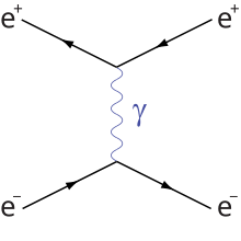 |
In quantum electrodynamics, Bhabha scattering is the electron-positron scattering process:
- e+e−→e+e−{displaystyle e^{+}e^{-}rightarrow e^{+}e^{-}}
- e+e−→e+e−{displaystyle e^{+}e^{-}rightarrow e^{+}e^{-}}

There are two leading-order Feynman diagrams contributing to this interaction: an annihilation process and a scattering process. Bhabha scattering is named after the Indian physicist Homi J. Bhabha.
The Bhabha scattering rate is used as a luminosity monitor in electron-positron colliders.
Contents
1 Differential cross section
1.1 Mandelstam variables
2 Deriving unpolarized cross section
2.1 Matrix elements
2.2 Square of matrix element
2.3 Scattering term (t-channel)
2.3.1 Magnitude squared of M
2.3.2 Sum over spins
2.4 Annihilation term (s-channel)
2.5 Solution
3 Simplifying steps
3.1 Completeness relations
3.2 Trace identities
4 Uses
5 References
Differential cross section
To leading order, the spin-averaged differential cross section for this process is
- dσd(cosθ)=πα2s(u2(1s+1t)2+(ts)2+(st)2){displaystyle {frac {mathrm {d} sigma }{mathrm {d} (cos theta )}}={frac {pi alpha ^{2}}{s}}left(u^{2}left({frac {1}{s}}+{frac {1}{t}}right)^{2}+left({frac {t}{s}}right)^{2}+left({frac {s}{t}}right)^{2}right),}
- dσd(cosθ)=πα2s(u2(1s+1t)2+(ts)2+(st)2){displaystyle {frac {mathrm {d} sigma }{mathrm {d} (cos theta )}}={frac {pi alpha ^{2}}{s}}left(u^{2}left({frac {1}{s}}+{frac {1}{t}}right)^{2}+left({frac {t}{s}}right)^{2}+left({frac {s}{t}}right)^{2}right),}

where s,t, and u are the Mandelstam variables, α{displaystyle alpha }

This cross section is calculated neglecting the electron mass relative to the collision energy and including only the contribution from photon exchange. This is a valid approximation at collision energies small compared to the mass scale of the Z boson, about 91 GeV; at higher energies the contribution from Z boson exchange also becomes important.
Mandelstam variables
In this article, the Mandelstam variables are defined by
s={displaystyle s=,}
(k+p)2={displaystyle (k+p)^{2}=,}
(k′+p′)2≈{displaystyle (k'+p')^{2}approx ,}
2k⋅p≈{displaystyle 2kcdot papprox ,}
2k′⋅p′{displaystyle 2k'cdot p',}
t={displaystyle t=,}
(k−k′)2={displaystyle (k-k')^{2}=,}
(p−p′)2≈{displaystyle (p-p')^{2}approx ,}
−2k⋅k′≈{displaystyle -2kcdot k'approx ,}
−2p⋅p′{displaystyle -2pcdot p',}
u={displaystyle u=,}
(k−p′)2={displaystyle (k-p')^{2}=,}
(p−k′)2≈{displaystyle (p-k')^{2}approx ,}
−2k⋅p′≈{displaystyle -2kcdot p'approx ,}
−2k′⋅p{displaystyle -2k'cdot p,}


where the approximations are for the high-energy (relativistic) limit.
Deriving unpolarized cross section
Matrix elements
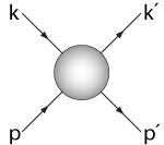
Both the scattering and annihilation diagrams contribute to the transition matrix element. By letting k and k' represent the four-momentum of the positron, while letting p and p' represent the four-momentum of the electron, and by using Feynman rules one can show the following diagrams give these matrix elements:


Where we use:
γμ{displaystyle gamma ^{mu },}are the Gamma matrices,
u, and u¯{displaystyle u, mathrm {and} {bar {u}},}are the four-component spinors for fermions, while
v, and v¯{displaystyle v, mathrm {and} {bar {v}},}are the four-component spinors for anti-fermions (see Four spinors).
(scattering)
(annihilation)
M={displaystyle {mathcal {M}}=,}
−e2(v¯kγμvk′)1(k−k′)2(u¯p′γμup){displaystyle -e^{2}left({bar {v}}_{k}gamma ^{mu }v_{k'}right){frac {1}{(k-k')^{2}}}left({bar {u}}_{p'}gamma _{mu }u_{p}right)}
+e2(v¯kγνup)1(k+p)2(u¯p′γνvk′){displaystyle +e^{2}left({bar {v}}_{k}gamma ^{nu }u_{p}right){frac {1}{(k+p)^{2}}}left({bar {u}}_{p'}gamma _{nu }v_{k'}right)}


Notice that there is a relative sign difference between the two diagrams.
Square of matrix element
To calculate the unpolarized cross section, one must average over the spins of the incoming particles (se- and se+ possible values) and sum over the spins of the outgoing particles. That is,
|M|2¯{displaystyle {overline {|{mathcal {M}}|^{2}}},}
=1(2se−+1)(2se++1)∑spins|M|2{displaystyle ={frac {1}{(2s_{e-}+1)(2s_{e+}+1)}}sum _{mathrm {spins} }|{mathcal {M}}|^{2},}
=14∑s=12∑s′=12∑r=12∑r′=12|M|2{displaystyle ={frac {1}{4}}sum _{s=1}^{2}sum _{s'=1}^{2}sum _{r=1}^{2}sum _{r'=1}^{2}|{mathcal {M}}|^{2},}


First, calculate |M|2{displaystyle |{mathcal {M}}|^{2},}
|M|2{displaystyle |{mathcal {M}}|^{2},}
e4|(v¯kγμvk′)(u¯p′γμup)(k−k′)2|2{displaystyle e^{4}left|{frac {({bar {v}}_{k}gamma ^{mu }v_{k'})({bar {u}}_{p'}gamma _{mu }u_{p})}{(k-k')^{2}}}right|^{2},}
(scattering)
−e4((v¯kγμvk′)(u¯p′γμup)(k−k′)2)∗((v¯kγνup)(u¯p′γνvk′)(k+p)2){displaystyle {}-e^{4}left({frac {({bar {v}}_{k}gamma ^{mu }v_{k'})({bar {u}}_{p'}gamma _{mu }u_{p})}{(k-k')^{2}}}right)^{*}left({frac {({bar {v}}_{k}gamma ^{nu }u_{p})({bar {u}}_{p'}gamma _{nu }v_{k'})}{(k+p)^{2}}}right),}
(interference)
−e4((v¯kγμvk′)(u¯p′γμup)(k−k′)2)((v¯kγνup)(u¯p′γνvk′)(k+p)2)∗{displaystyle {}-e^{4}left({frac {({bar {v}}_{k}gamma ^{mu }v_{k'})({bar {u}}_{p'}gamma _{mu }u_{p})}{(k-k')^{2}}}right)left({frac {({bar {v}}_{k}gamma ^{nu }u_{p})({bar {u}}_{p'}gamma _{nu }v_{k'})}{(k+p)^{2}}}right)^{*},}
(interference)
+e4|(v¯kγνup)(u¯p′γνvk′)(k+p)2|2{displaystyle {}+e^{4}left|{frac {({bar {v}}_{k}gamma ^{nu }u_{p})({bar {u}}_{p'}gamma _{nu }v_{k'})}{(k+p)^{2}}}right|^{2},}
(annihilation)


Scattering term (t-channel)
Magnitude squared of M
|M|2{displaystyle |{mathcal {M}}|^{2},}
=e4(k−k′)4((v¯kγμvk′)(u¯p′γμup))∗((v¯kγνvk′)(u¯p′γνup)){displaystyle ={frac {e^{4}}{(k-k')^{4}}}{Big (}({bar {v}}_{k}gamma ^{mu }v_{k'})({bar {u}}_{p'}gamma _{mu }u_{p}){Big )}^{*}{Big (}({bar {v}}_{k}gamma ^{nu }v_{k'})({bar {u}}_{p'}gamma _{nu }u_{p}){Big )},}
(1){displaystyle (1),}
=e4(k−k′)4((v¯kγμvk′)∗(u¯p′γμup)∗)((v¯kγνvk′)(u¯p′γνup)){displaystyle ={frac {e^{4}}{(k-k')^{4}}}{Big (}({bar {v}}_{k}gamma ^{mu }v_{k'})^{*}({bar {u}}_{p'}gamma _{mu }u_{p})^{*}{Big )}{Big (}({bar {v}}_{k}gamma ^{nu }v_{k'})({bar {u}}_{p'}gamma _{nu }u_{p}){Big )},}
(2){displaystyle (2),}
(complex conjugate will flip order)
=e4(k−k′)4((v¯k′γμvk)(u¯pγμup′))((v¯kγνvk′)(u¯p′γνup)){displaystyle ={frac {e^{4}}{(k-k')^{4}}}{Big (}left({bar {v}}_{k'}gamma ^{mu }v_{k}right)left({bar {u}}_{p}gamma _{mu }u_{p'}right){Big )}{Big (}left({bar {v}}_{k}gamma ^{nu }v_{k'}right)left({bar {u}}_{p'}gamma _{nu }u_{p}right){Big )},}
(3){displaystyle (3),}
(move terms that depend on same momentum to be next to each other)
=e4(k−k′)4(v¯k′γμvk)(v¯kγνvk′)(u¯pγμup′)(u¯p′γνup){displaystyle ={frac {e^{4}}{(k-k')^{4}}}left({bar {v}}_{k'}gamma ^{mu }v_{k}right)left({bar {v}}_{k}gamma ^{nu }v_{k'}right)left({bar {u}}_{p}gamma _{mu }u_{p'}right)left({bar {u}}_{p'}gamma _{nu }u_{p}right),}
(4){displaystyle (4),}


Sum over spins
Next, we'd like to sum over spins of all four particles. Let s and s' be the spin of the electron and r and r' be the spin of the positron.
∑spins|M|2{displaystyle sum _{mathrm {spins} }|{mathcal {M}}|^{2},}
=e4(k−k′)4(∑r′v¯k′γμ(∑rvkv¯k)γνvk′)(∑su¯pγμ(∑s′up′u¯p′)γνup){displaystyle ={frac {e^{4}}{(k-k')^{4}}}left(sum _{r'}{bar {v}}_{k'}gamma ^{mu }(sum _{r}v_{k}{bar {v}}_{k})gamma ^{nu }v_{k'}right)left(sum _{s}{bar {u}}_{p}gamma _{mu }(sum _{s'}{u_{p'}{bar {u}}_{p'}})gamma _{nu }u_{p}right),}
(5){displaystyle (5),}
=e4(k−k′)4Tr((∑r′vk′v¯k′)γμ(∑rvkv¯k)γν)Tr((∑supu¯p)γμ(∑s′up′u¯p′)γν){displaystyle ={frac {e^{4}}{(k-k')^{4}}}operatorname {Tr} left({Big (}sum _{r'}v_{k'}{bar {v}}_{k'}{Big )}gamma ^{mu }{Big (}sum _{r}v_{k}{bar {v}}_{k}{Big )}gamma ^{nu }right)operatorname {Tr} left({Big (}sum _{s}u_{p}{bar {u}}_{p}{Big )}gamma _{mu }{Big (}sum _{s'}{u_{p'}{bar {u}}_{p'}}{Big )}gamma _{nu }right),}
(6){displaystyle (6),}
(now use Completeness relations)
=e4(k−k′)4Tr((k/′−m)γμ(k/−m)γν)⋅Tr((p/′+m)γμ(p/+m)γν){displaystyle ={frac {e^{4}}{(k-k')^{4}}}operatorname {Tr} left((k!!!/'-m)gamma ^{mu }(k!!!/-m)gamma ^{nu }right)cdot operatorname {Tr} left((p!!!/'+m)gamma _{mu }(p!!!/+m)gamma _{nu }right),}
(7){displaystyle (7),}
(now use Trace identities)
=e4(k−k′)4(4(k′μkν−(k′⋅k)ημν+k′νkμ)+4m2ημν)(4(p′μpν−(p′⋅p)ημν+pν′pμ)+4m2ημν){displaystyle ={frac {e^{4}}{(k-k')^{4}}}left(4left({k'}^{mu }k^{nu }-(k'cdot k)eta ^{mu nu }+k'^{nu }k^{mu }right)+4m^{2}eta ^{mu nu }right)left(4left({p'}_{mu }p_{nu }-(p'cdot p)eta _{mu nu }+p'_{nu }p_{mu }right)+4m^{2}eta _{mu nu }right),}
(8){displaystyle (8),}
=32e4(k−k′)4((k′⋅p′)(k⋅p)+(k′⋅p)(k⋅p′)−m2p′⋅p−m2k′⋅k+2m4){displaystyle ={frac {32{e^{4}}}{(k-k')^{4}}}left((k'cdot p')(kcdot p)+(k'cdot p)(kcdot p')-m^{2}p'cdot p-m^{2}k'cdot k+2m^{4}right),}
(9){displaystyle (9),}


Now that is the exact form, in the case of electrons one is usually interested in energy scales that far exceed the electron mass. Neglecting the electron mass yields the simplified form:
14∑spins|M|2{displaystyle {frac {1}{4}}sum _{mathrm {spins} }|{mathcal {M}}|^{2},}
=32e44(k−k′)4((k′⋅p′)(k⋅p)+(k′⋅p)(k⋅p′)){displaystyle ={frac {32e^{4}}{4(k-k')^{4}}}left((k'cdot p')(kcdot p)+(k'cdot p)(kcdot p')right),}
(use the Mandelstam variables in this relativistic limit)
=8e4t2(12s12s+12u12u){displaystyle ={frac {8e^{4}}{t^{2}}}left({tfrac {1}{2}}s{tfrac {1}{2}}s+{tfrac {1}{2}}u{tfrac {1}{2}}uright),}
=2e4s2+u2t2{displaystyle =2e^{4}{frac {s^{2}+u^{2}}{t^{2}}},}


Annihilation term (s-channel)
The process for finding the annihilation term is similar to the above. Since the two diagrams are related by crossing symmetry, and the initial and final state particles are the same, it is sufficient to permute the momenta, yielding
14∑spins|M|2{displaystyle {frac {1}{4}}sum _{mathrm {spins} }|{mathcal {M}}|^{2},}
=32e44(k+p)4((k⋅k′)(p⋅p′)+(k′⋅p)(k⋅p′)){displaystyle ={frac {32e^{4}}{4(k+p)^{4}}}left((kcdot k')(pcdot p')+(k'cdot p)(kcdot p')right),}
=8e4s2(12t12t+12u12u){displaystyle ={frac {8e^{4}}{s^{2}}}left({tfrac {1}{2}}t{tfrac {1}{2}}t+{tfrac {1}{2}}u{tfrac {1}{2}}uright),}
=2e4t2+u2s2{displaystyle =2e^{4}{frac {t^{2}+u^{2}}{s^{2}}},}


(This is proportional to
(1+cos2θ){displaystyle (1+cos ^{2}theta )}
where θ{displaystyle theta }

Solution
Evaluating the interference term along the same lines and adding the three terms yields the final result
- |M|2¯2e4=u2+s2t2+2u2st+u2+t2s2{displaystyle {frac {overline {|{mathcal {M}}|^{2}}}{2e^{4}}}={frac {u^{2}+s^{2}}{t^{2}}}+{frac {2u^{2}}{st}}+{frac {u^{2}+t^{2}}{s^{2}}},}
- |M|2¯2e4=u2+s2t2+2u2st+u2+t2s2{displaystyle {frac {overline {|{mathcal {M}}|^{2}}}{2e^{4}}}={frac {u^{2}+s^{2}}{t^{2}}}+{frac {2u^{2}}{st}}+{frac {u^{2}+t^{2}}{s^{2}}},}

Simplifying steps
Completeness relations
The completeness relations for the four-spinors u and v are
- ∑s=1,2up(s)u¯p(s)=p/+m{displaystyle sum _{s=1,2}{u_{p}^{(s)}{bar {u}}_{p}^{(s)}}=p!!!/+m,}
- ∑s=1,2vp(s)v¯p(s)=p/−m{displaystyle sum _{s=1,2}{v_{p}^{(s)}{bar {v}}_{p}^{(s)}}=p!!!/-m,}
- ∑s=1,2up(s)u¯p(s)=p/+m{displaystyle sum _{s=1,2}{u_{p}^{(s)}{bar {u}}_{p}^{(s)}}=p!!!/+m,}
- where
p/=γμpμ{displaystyle p!!!/=gamma ^{mu }p_{mu },}(see Feynman slash notation)
- u¯=u†γ0{displaystyle {bar {u}}=u^{dagger }gamma ^{0},}


Trace identities
Main article: Trace identities
To simplify the trace of the Dirac gamma matrices, one must use trace identities. Three used in this article are:
- The Trace of any product of an odd number of γμ{displaystyle gamma _{mu },}
's is zero
- Tr(γμγν)=4ημν{displaystyle operatorname {Tr} (gamma ^{mu }gamma ^{nu })=4eta ^{mu nu }}
- Tr(γργμγσγν)=4(ηρμησν−ηρσημν+ηρνημσ){displaystyle operatorname {Tr} left(gamma _{rho }gamma _{mu }gamma _{sigma }gamma _{nu }right)=4left(eta _{rho mu }eta _{sigma nu }-eta _{rho sigma }eta _{mu nu }+eta _{rho nu }eta _{mu sigma }right),}


Using these two one finds that, for example,
Tr((p/′+m)γμ(p/+m)γν){displaystyle operatorname {Tr} left((p!!!/'+m)gamma _{mu }(p!!!/+m)gamma _{nu }right),}
=Tr(p/′γμp/γν)+Tr(mγμp/γν){displaystyle =operatorname {Tr} left(p!!!/'gamma _{mu }p!!!/gamma _{nu }right)+operatorname {Tr} left(mgamma _{mu }p!!!/gamma _{nu }right),}
+Tr(p/′γμmγν)+Tr(m2γμγν){displaystyle +operatorname {Tr} left(p!!!/'gamma _{mu }mgamma _{nu }right)+operatorname {Tr} left(m^{2}gamma _{mu }gamma _{nu }right),}
(the two middle terms are zero because of (1))
=Tr(p/′γμp/γν)+m2Tr(γμγν){displaystyle =operatorname {Tr} left(p!!!/'gamma _{mu }p!!!/gamma _{nu }right)+m^{2}operatorname {Tr} left(gamma _{mu }gamma _{nu }right),}
(use identity (2) for the term on the right)
=p′ρpσTr(γργμγσγν)+m2⋅4ημν{displaystyle ={p'}^{rho }p^{sigma }operatorname {Tr} left(gamma _{rho }gamma _{mu }gamma _{sigma }gamma _{nu }right)+m^{2}cdot 4eta _{mu nu },}
(now use identity (3) for the term on the left)
=p′ρpσ4(ηρμησν−ηρσημν+ηρνημσ)+4m2ημν{displaystyle ={p'}^{rho }p^{sigma }4left(eta _{rho mu }eta _{sigma nu }-eta _{rho sigma }eta _{mu nu }+eta _{rho nu }eta _{mu sigma }right)+4m^{2}eta _{mu nu },}
=4(p′μpν−(p′⋅p)ημν+pν′pμ)+4m2ημν{displaystyle =4left({p'}_{mu }p_{nu }-(p'cdot p)eta _{mu nu }+p'_{nu }p_{mu }right)+4m^{2}eta _{mu nu },}


Uses
Bhabha scattering has been used as a luminosity monitor in a number of e+e− collider physics experiments. The accurate measurement of luminosity is necessary for accurate measurements of cross sections.
Small-angle Bhabha scattering was used to measure the luminosity of the 1993 run of the Stanford Large Detector (SLD), with a relative uncertainty of less than 0.5%.[1]
Electron-positron colliders operating in the region of the low-lying hadronic resonances (about 1 GeV to 10 GeV), such as the Beijing Electron Synchrotron (BES) and the Belle and BaBar "B-factory" experiments, use large-angle Bhabha scattering as a luminosity monitor. To achieve the desired precision at the 0.1% level, the experimental measurements must be compared to a theoretical calculation including next-to-leading-order radiative corrections.[2] The high-precision measurement of the total hadronic cross section at these low energies is a crucial input into the theoretical calculation of the anomalous magnetic dipole moment of the muon, which is used to constrain supersymmetry and other models of physics beyond the Standard Model.
References
^ "a Study of Small Angle Radiative Bhabha Scattering and Measurement of the Lumino". Bibcode:1995PhDT.......160W..mw-parser-output cite.citation{font-style:inherit}.mw-parser-output .citation q{quotes:"""""""'""'"}.mw-parser-output .citation .cs1-lock-free a{background:url("//upload.wikimedia.org/wikipedia/commons/thumb/6/65/Lock-green.svg/9px-Lock-green.svg.png")no-repeat;background-position:right .1em center}.mw-parser-output .citation .cs1-lock-limited a,.mw-parser-output .citation .cs1-lock-registration a{background:url("//upload.wikimedia.org/wikipedia/commons/thumb/d/d6/Lock-gray-alt-2.svg/9px-Lock-gray-alt-2.svg.png")no-repeat;background-position:right .1em center}.mw-parser-output .citation .cs1-lock-subscription a{background:url("//upload.wikimedia.org/wikipedia/commons/thumb/a/aa/Lock-red-alt-2.svg/9px-Lock-red-alt-2.svg.png")no-repeat;background-position:right .1em center}.mw-parser-output .cs1-subscription,.mw-parser-output .cs1-registration{color:#555}.mw-parser-output .cs1-subscription span,.mw-parser-output .cs1-registration span{border-bottom:1px dotted;cursor:help}.mw-parser-output .cs1-ws-icon a{background:url("//upload.wikimedia.org/wikipedia/commons/thumb/4/4c/Wikisource-logo.svg/12px-Wikisource-logo.svg.png")no-repeat;background-position:right .1em center}.mw-parser-output code.cs1-code{color:inherit;background:inherit;border:inherit;padding:inherit}.mw-parser-output .cs1-hidden-error{display:none;font-size:100%}.mw-parser-output .cs1-visible-error{font-size:100%}.mw-parser-output .cs1-maint{display:none;color:#33aa33;margin-left:0.3em}.mw-parser-output .cs1-subscription,.mw-parser-output .cs1-registration,.mw-parser-output .cs1-format{font-size:95%}.mw-parser-output .cs1-kern-left,.mw-parser-output .cs1-kern-wl-left{padding-left:0.2em}.mw-parser-output .cs1-kern-right,.mw-parser-output .cs1-kern-wl-right{padding-right:0.2em}
^ Carloni Calame, C. M; Lunardini, C; Montagna, G; Nicrosini, O; Piccinini, F (2000). "Large-angle Bhabha scattering and luminosity at flavour factories". Nuclear Physics B. 584: 459–479. arXiv:hep-ph/0003268. Bibcode:2000NuPhB.584..459C. doi:10.1016/S0550-3213(00)00356-4.
Halzen, Francis; Martin, Alan (1984). Quarks & Leptons: An Introductory Course in Modern Particle Physics. John Wiley & Sons. ISBN 0-471-88741-2.
Peskin, Michael E.; Schroeder, Daniel V. (1994). An Introduction to Quantum Field Theory. Perseus Publishing. ISBN 0-201-50397-2.
- Bhabha scattering on arxiv.org


Comments
Post a Comment