Elliptic curve

Not to be confused with Ellipse.

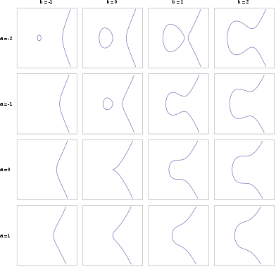
A catalog of elliptic curves. Region shown is [−3,3]² (For (a, b) = (0, 0) the function is not smooth and therefore not an elliptic curve.)

Algebraic structure → Group theory Group theory
Basic notions Subgroup Normal subgroup Quotient group (Semi-)direct product Group homomorphisms kernel image direct sum wreath product simple finite infinite continuous multiplicative additive cyclic abelian dihedral nilpotent solvable List of group theory topics
Finite groups Classification of finite simple groups cyclic alternating Lie type sporadic Lagrange's theorem Sylow theorems Hall's theorem p-group Elementary abelian group Frobenius group Schur multiplier Symmetric group Sn Klein four-group V Dihedral group Dn Quaternion group Q Dicyclic group Dicn
Discrete groups Lattices Integers (Z) Free group Modular groups PSL(2,Z) SL(2,Z) Arithmetic group Lattice Hyperbolic group
Topological and Lie groups Solenoid Circle General linear GL(n) Special linear SL(n) Orthogonal O(n) Euclidean E(n) Special orthogonal SO(n) Unitary U(n) Special unitary SU(n) Symplectic Sp(n) G2 F4 E6 E7 E8 Lorentz Poincaré Conformal Diffeomorphism Loop Infinite dimensional Lie group O(∞) SU(∞) Sp(∞)
Algebraic groups Linear algebraic group Reductive group Abelian variety Elliptic curve
v t e

In mathematics, an elliptic curve is a plane algebraic curve defined by an equation of the form

y2=x3+ax+b{displaystyle y^{2}=x^{3}+ax+b}

which is non-singular; that is, the curve has no cusps or self-intersections. (When the coefficient field has characteristic 2 or 3, the above equation is not quite general enough to comprise all non-singular cubic curves; see § Elliptic curves over a general field below.)

Formally, an elliptic curve is a smooth, projective, algebraic curve of genus one, on which there is a specified point O. An elliptic curve is an abelian variety – that is, it has a multiplication defined algebraically, with respect to which it is an abelian group – and O serves as the identity element. Often the curve itself, without O specified, is called an elliptic curve; the point O is often taken to be the curve's "point at infinity" in the projective plane.

If y² = P(x), where P is any polynomial of degree three in x with no repeated roots, the solution set is a nonsingular plane curve of genus one, an elliptic curve. If P has degree four and is square-free this equation again describes a plane curve of genus one; however, it has no natural choice of identity element. More generally, any algebraic curve of genus one, for example from the intersection of two quadric surfaces embedded in three-dimensional projective space, is called an elliptic curve, provided that it has at least one rational point to act as the identity.

Using the theory of elliptic functions, it can be shown that elliptic curves defined over the complex numbers correspond to embeddings of the torus into the complex projective plane. The torus is also an abelian group, and in fact this correspondence is also a group isomorphism.

Elliptic curves are especially important in number theory, and constitute a major area of current research; for example, they were used in the proof, by Andrew Wiles, of Fermat's Last Theorem. They also find applications in elliptic curve cryptography (ECC) and integer factorization.

An elliptic curve is not an ellipse: see elliptic integral for the origin of the term. Topologically, a complex elliptic curve is a torus.

Contents

• 
  1 Elliptic curves over the real numbers
  


• 
  2 The group law
  


• 
  3 Elliptic curves over the complex numbers
  


• 
  4 Elliptic curves over the rational numbers
  
  
  
  • 
    4.1 The structure of rational points
    
  
  
  • 
    4.2 The Birch and Swinnerton-Dyer conjecture
    
  
  
  • 
    4.3 The modularity theorem and its application to Fermat's Last Theorem
    
  
  
  • 
    4.4 Integral points
    
  
  
  • 
    4.5 Generalization to number fields
    
  
  
  
  


• 
  5 Elliptic curves over a general field
  


• 
  6 Isogeny
  


• 
  7 Elliptic curves over finite fields
  


• 
  8 Applications
  


• 
  9 Algorithms that use elliptic curves
  


• 
  10 Alternative representations of elliptic curves
  


• 
  11 See also
  


• 
  12 Notes
  


• 
  13 References
  


• 
  14 External links
  

Elliptic curves over the real numbers

Graphs of curves y² = x³ − x and y² = x³ − x + 1

Although the formal definition of an elliptic curve is fairly technical and requires some background in algebraic geometry, it is possible to describe some features of elliptic curves over the real numbers using only introductory algebra and geometry.

In this context, an elliptic curve is a plane curve defined by an equation of the form

y2=x3+ax+b{displaystyle y^{2}=x^{3}+ax+b}

where a and b are real numbers. This type of equation is called a Weierstrass equation.

The definition of elliptic curve also requires that the curve be non-singular. Geometrically, this means that the graph has no cusps, self-intersections, or isolated points. Algebraically, this holds if and only if the discriminant

Δ=−16(4a3+27b2){displaystyle Delta =-16(4a^{3}+27b^{2})}

is not equal to zero. (Although the factor −16 is irrelevant to whether or not the curve is non-singular, this definition of the discriminant is useful in a more advanced study of elliptic curves.)

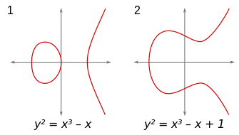
The (real) graph of a non-singular curve has two components if its discriminant is positive, and one component if it is negative. For example, in the graphs shown in figure to the right, the discriminant in the first case is 64, and in the second case is −368.

The group law

When working in the projective plane, we can define a group structure on any smooth cubic curve. In Weierstrass normal form, such a curve will have an additional point at infinity, O, at the homogeneous coordinates [0:1:0] which serves as the identity of the group.

Since the curve is symmetrical about the x-axis, given any point P, we can take −P to be the point opposite it. We take −O to be just O.

If P and Q are two points on the curve, then we can uniquely describe a third point, P + Q, in the following way. First, draw the line that intersects P and Q. This will generally intersect the cubic at a third point, R. We then take P + Q to be −R, the point opposite R.

This definition for addition works except in a few special cases related to the point at infinity and intersection multiplicity. The first is when one of the points is O. Here, we define P + O = P = O + P, making O the identity of the group. Next, if P and Q are opposites of each other, we define P + Q = O. Lastly, if P = Q we only have one point, thus we can't define the line between them. In this case, we use the tangent line to the curve at this point as our line. In most cases, the tangent will intersect a second point R and we can take its opposite. However, if P happens to be an inflection point (a point where the concavity of the curve changes), we take R to be P itself and P + P is simply the point opposite itself.

For a cubic curve not in Weierstrass normal form, we can still define a group structure by designating one of its nine inflection points as the identity O. In the projective plane, each line will intersect a cubic at three points when accounting for multiplicity. For a point P, −P is defined as the unique third point on the line passing through O and P. Then, for any P and Q, P + Q is defined as −R where R is the unique third point on the line containing P and Q.

Let K be a field over which the curve is defined (i.e., the coefficients of the defining equation or equations of the curve are in K) and denote the curve by E. Then the K-rational points of E are the points on E whose coordinates all lie in K, including the point at infinity. The set of K-rational points is denoted by E(K). It, too, forms a group, because properties of polynomial equations show that if P is in E(K), then −P is also in E(K), and if two of P, Q, and R are in E(K), then so is the third. Additionally, if K is a subfield of L, then E(K) is a subgroup of E(L).

The above group can be described algebraically as well as geometrically. Given the curve y² = x³ + ax + b over the field K (whose characteristic we assume to be neither 2 nor 3), and points P = (x_P, y_P) and Q = (x_Q, y_Q) on the curve, assume first that x_P ≠ x_Q (first pane below). Let y = sx + d be the line that intersects P and Q, which has the following slope:

s=yP−yQxP−xQ{displaystyle s={frac {y_{P}-y_{Q}}{x_{P}-x_{Q}}}}

Since K is a field, s is well-defined. The line equation and the curve equation have an identical y in the points x_P, x_Q, and x_R.

(sx+d)2=x3+ax+b{displaystyle (sx+d)^{2}=x^{3}+ax+b}

which is equivalent to 0=x3−s2x2−2xd+ax+b−d2{displaystyle 0=x^{3}-s^{2}x^{2}-2xd+ax+b-d^{2}}. We know that this equation has its roots in exactly the same x-values as

(x−xP)(x−xQ)(x−xR)=x3+x2(−xP−xQ−xR)+x(xPxQ+xPxR+xQxR)−xPxQxR{displaystyle (x-x_{P})(x-x_{Q})(x-x_{R})=x^{3}+x^{2}(-x_{P}-x_{Q}-x_{R})+x(x_{P}x_{Q}+x_{P}x_{R}+x_{Q}x_{R})-x_{P}x_{Q}x_{R}}

We equate the coefficient for x² and solve for x_R. y_R follows from the line equation. This defines R = (x_R, y_R) = −(P + Q) with

xR=s2−xP−xQyR=yP+s(xR−xP){displaystyle {begin{aligned}x_{R}&=s^{2}-x_{P}-x_{Q}\y_{R}&=y_{P}+s(x_{R}-x_{P})end{aligned}}}

If x_P = x_Q, then there are two options: if y_P = −y_Q (third and fourth panes below), including the case where y_P = y_Q = 0 (fourth pane), then the sum is defined as 0; thus, the inverse of each point on the curve is found by reflecting it across the x-axis. If y_P = y_Q ≠ 0, then Q = P and R = (x_R, y_R) = −(P + P) = −2P = −2Q (second pane below with P shown for R) is given by

s=3xP2+a2yPxR=s2−2xPyR=yP+s(xR−xP){displaystyle {begin{aligned}s&={frac {3{x_{P}}^{2}+a}{2y_{P}}}\x_{R}&=s^{2}-2x_{P}\y_{R}&=y_{P}+s(x_{R}-x_{P})end{aligned}}}

Elliptic curves over the complex numbers

An elliptic curve over the complex numbers is obtained as a quotient of the complex plane by a lattice Λ, here spanned by two fundamental periods ω₁ and ω₂. The four-torsion is also shown, corresponding to the lattice 1/4 Λ containing Λ.

The formulation of elliptic curves as the embedding of a torus in the complex projective plane follows naturally from a curious property of Weierstrass's elliptic functions. These functions and their first derivative are related by the formula

℘′(z)2=4℘(z)3−g2℘(z)−g3{displaystyle wp '(z)^{2}=4wp (z)^{3}-g_{2}wp (z)-g_{3}}

Here, g₂ and g₃ are constants; ℘(z){displaystyle wp (z)} is the Weierstrass elliptic function and ℘′(z){displaystyle wp '(z)} its derivative. It should be clear that this relation is in the form of an elliptic curve (over the complex numbers). The Weierstrass functions are doubly periodic; that is, they are periodic with respect to a lattice Λ; in essence, the Weierstrass functions are naturally defined on a torus T = C/Λ. This torus may be embedded in the complex projective plane by means of the map

z↦[1:℘(z):℘′(z)/2]{displaystyle zmapsto [1:wp (z):wp '(z)/2]}

This map is a group isomorphism of the torus (considered with its natural group structure) with the chord-and-tangent group law on the cubic curve which is the image of this map. It is also an isomorphism of Riemann surfaces from the torus to the cubic curve, so topologically, an elliptic curve is a torus. If the lattice Λ is related by multiplication by a non-zero complex number c to a lattice cΛ, then the corresponding curves are isomorphic. Isomorphism classes of elliptic curves are specified by the j-invariant.

The isomorphism classes can be understood in a simpler way as well. The constants g₂ and g₃, called the modular invariants, are uniquely determined by the lattice, that is, by the structure of the torus. However, the complex numbers form the splitting field for polynomials with real coefficients, and so the elliptic curve may be written as

y2=x(x−1)(x−λ){displaystyle y^{2}=x(x-1)(x-lambda )}

One finds that

g2=433(λ2−λ+1){displaystyle g_{2}={frac {sqrt[{3}]{4}}{3}}(lambda ^{2}-lambda +1)}

and

g3=127(λ+1)(2λ2−5λ+2){displaystyle g_{3}={frac {1}{27}}(lambda +1)(2lambda ^{2}-5lambda +2)}

so that the modular discriminant is

Δ=g23−27g32=λ2(λ−1)2{displaystyle Delta =g_{2}^{3}-27g_{3}^{2}=lambda ^{2}(lambda -1)^{2}}

Here, λ is sometimes called the modular lambda function.

Note that the uniformization theorem implies that every compact Riemann surface of genus one can be represented as a torus.

This also allows an easy understanding of the torsion points on an elliptic curve: if the lattice Λ is spanned by the fundamental periods ω₁ and ω₂, then the n-torsion points are the (equivalence classes of) points of the form

anω1+bnω2{displaystyle {frac {a}{n}}omega _{1}+{frac {b}{n}}omega _{2}}

for a and b integers in the range from 0 to n−1.

Over the complex numbers, every elliptic curve has nine inflection points. Every line through two of these points also passes through a third inflection point; the nine points and 12 lines formed in this way form a realization of the Hesse configuration.

Elliptic curves over the rational numbers

A curve E defined over the field of rational numbers is also defined over the field of real numbers. Therefore, the law of addition (of points with real coordinates) by the tangent and secant method can be applied to E. The explicit formulae show that the sum of two points P and Q with rational coordinates has again rational coordinates, since the line joining P and Q has rational coefficients. This way, one shows that the set of rational points of E forms a subgroup of the group of real points of E. As this group, it is an abelian group, that is, P + Q = Q + P.

The structure of rational points

The most important result is that all points can be constructed by the method of tangents and secants starting with a finite number of points. More precisely^[1] the Mordell–Weil theorem states that the group E(Q) is a finitely generated (abelian) group. By the fundamental theorem of finitely generated abelian groups it is therefore a finite direct sum of copies of Z and finite cyclic groups.

The proof of that theorem^[2] rests on two ingredients: first, one shows that for any integer m > 1, the quotient group E(Q)/mE(Q) is finite (weak Mordell–Weil theorem). Second, introducing a height function h on the rational points E(Q) defined by h(P₀) = 0 and h(P) = log max(|p|, |q|) if P (unequal to the point at infinity P₀) has as abscissa the rational number x = p/q (with coprime p and q). This height function h has the property that h(mP) grows roughly like the square of m. Moreover, only finitely many rational points with height smaller than any constant exist on E.

The proof of the theorem is thus a variant of the method of infinite descent^[3] and relies on the repeated application of Euclidean divisions on E: let P ∈ E(Q) be a rational point on the curve, writing P as the sum 2P₁ + Q₁ where Q₁ is a fixed representant of P in E(Q)/2E(Q), the height of P₁ is about 1/4 of the one of P (more generally, replacing 2 by any m > 1, and 1/4 by 1/m²). Redoing the same with P₁, that is to say P₁ = 2P₂ + Q₂, then P₂ = 2P₃ + Q₃, etc. finally expresses P as an integral linear combination of points Q_i and of points whose height is bounded by a fixed constant chosen in advance: by the weak Mordell–Weil theorem and the second property of the height function P is thus expressed as an integral linear combination of a finite number of fixed points.

So far, the theorem is not effective since there is no known general procedure for determining the representants of E(Q)/mE(Q).

The rank of E(Q), that is the number of copies of Z in E(Q) or, equivalently, the number of independent points of infinite order, is called the rank of E. The Birch and Swinnerton-Dyer conjecture is concerned with determining the rank. One conjectures that it can be arbitrarily large, even if only examples with relatively small rank are known. The elliptic curve with biggest exactly known rank is

y² + xy + y = x³ − x² + 31368015812338065133318565292206590792820353345x + 302038802698566087335643188429543498624522041683874493555186062568159847

It has rank 19, found by Noam Elkies in 2009.^[4] Curves of rank at least 28 are known, but their rank is not exactly known.

As for the groups constituting the torsion subgroup of E(Q), the following is known:^[5] the torsion subgroup of E(Q) is one of the 15 following groups (a theorem due to Barry Mazur): Z/NZ for N = 1, 2, ..., 10, or 12, or Z/2Z × Z/2NZ with N = 1, 2, 3, 4. Examples for every case are known. Moreover, elliptic curves whose Mordell–Weil groups over Q have the same torsion groups belong to a parametrized family.^[6]

The Birch and Swinnerton-Dyer conjecture

Main article: Birch and Swinnerton-Dyer conjecture

The Birch and Swinnerton-Dyer conjecture (BSD) is one of the Millennium problems of the Clay Mathematics Institute. The conjecture relies on analytic and arithmetic objects defined by the elliptic curve in question.

At the analytic side, an important ingredient is a function of a complex variable, L, the Hasse–Weil zeta function of E over Q. This function is a variant of the Riemann zeta function and Dirichlet L-functions. It is defined as an Euler product, with one factor for every prime number p.

For a curve E over Q given by a minimal equation

y2+a1xy+a3y=x3+a2x2+a4x+a6{displaystyle y^{2}+a_{1}xy+a_{3}y=x^{3}+a_{2}x^{2}+a_{4}x+a_{6}}

with integral coefficients ai{displaystyle a_{i}}, reducing the coefficients modulo p defines an elliptic curve over the finite field F_p (except for a finite number of primes p, where the reduced curve has a singularity and thus fails to be elliptic, in which case E is said to be of bad reduction at p).

The zeta function of an elliptic curve over a finite field F_p is, in some sense, a generating function assembling the information of the number of points of E with values in the finite field extensions F_pⁿ of F_p. It is given by^[7]

Z(E(Fp))=exp⁡(∑card[E(Fpn)]Tnn){displaystyle Z(E(mathbf {F} _{p}))=exp left(sum mathrm {card} left[E({mathbf {F} }_{p^{n}})right]{frac {T^{n}}{n}}right)}

The interior sum of the exponential resembles the development of the logarithm and, in fact, the so-defined zeta function is a rational function:

Z(E(Fp))=1−apT+pT2(1−T)(1−pT),{displaystyle Z(E(mathbf {F} _{p}))={frac {1-a_{p}T+pT^{2}}{(1-T)(1-pT)}},}

where the 'trace of Frobenius' term^[8]ap{displaystyle a_{p}} is defined to be the (negative of) the difference between the number of points on the elliptic curve E{displaystyle E} over Fp{displaystyle mathbb {F} _{p}} and the 'expected' number p+1{displaystyle p+1}, viz.:

ap=p+1−#E(Fp).{displaystyle a_{p}=p+1-#E(mathbb {F} _{p}).}

Two points to note about this quantity: (i) DO NOT confuse these ap{displaystyle a_{p}} with the ai{displaystyle a_{i}} in the definition of the curve E{displaystyle E} above: this is just an unfortunate clash of notation; (ii) we may define the same quantities and functions over an arbitrary finite field of characteristic p{displaystyle p}, with q=pn{displaystyle q=p^{n}} replacing p{displaystyle p} everywhere.

The Hasse–Weil zeta function of E over Q is then defined by collecting this information together, for all primes p. It is defined by

L(E(Q),s)=∏p(1−app−s+ε(p)p1−2s)−1{displaystyle L(E(mathbf {Q} ),s)=prod _{p}left(1-a_{p}p^{-s}+varepsilon (p)p^{1-2s}right)^{-1}}

where ε(p) = 1 if E has good reduction at p and 0 otherwise (in which case a_p is defined differently from the method above: see Silverman (1986) below).

This product converges for Re(s) > 3/2 only. Hasse's conjecture affirms that the L-function admits an analytic continuation to the whole complex plane and satisfies a functional equation relating, for any s, L(E, s) to L(E, 2 − s). In 1999 this was shown to be a consequence of the proof of the Shimura–Taniyama–Weil conjecture, which asserts that every elliptic curve over Q is a modular curve, which implies that its L-function is the L-function of a modular form whose analytic continuation is known.

One can therefore speak about the values of L(E, s) at any complex number s. The Birch–Swinnerton-Dyer conjecture relates the arithmetic of the curve to the behavior of its L-function at s = 1. More precisely, it affirms that the order of the L-function at s = 1 equals the rank of E and predicts the leading term of the Laurent series of L(E, s) at that point in terms of several quantities attached to the elliptic curve.

Much like the Riemann hypothesis, this conjecture has multiple consequences, including the following two:

• Let n be an odd square-free integer. Assuming the Birch and Swinnerton-Dyer conjecture, n is the area of a right triangle with rational side lengths (a congruent number) if and only if the number of triplets of integers (x, y, z) satisfying 2x2+y2+8z2=n{displaystyle 2x^{2}+y^{2}+8z^{2}=n} is twice the number of triples satisfying 2x2+y2+32z2=n{displaystyle 2x^{2}+y^{2}+32z^{2}=n}. This statement, due to Tunnell, is related to the fact that n is a congruent number if and only if the elliptic curve y2=x3−n2x{displaystyle y^{2}=x^{3}-n^{2}x} has a rational point of infinite order (thus, under the Birch and Swinnerton-Dyer conjecture, its L-function has a zero at 1). The interest in this statement is that the condition is easily verified.^[9]
  


• In a different direction, certain analytic methods allow for an estimation of the order of zero in the center of the critical strip of families of L-functions. Admitting the BSD conjecture, these estimations correspond to information about the rank of families of elliptic curves in question. For example:^[10] suppose the generalized Riemann hypothesis and the BSD conjecture, the average rank of curves given by y2=x3+ax+b{displaystyle y^{2}=x^{3}+ax+b} is smaller than 2.

The modularity theorem and its application to Fermat's Last Theorem

Main article: Modularity theorem

The modularity theorem, once known as the Taniyama–Shimura–Weil conjecture, states that every elliptic curve E over Q is a modular curve, that is to say, its Hasse–Weil zeta function is the L-function of a modular form of weight 2 and level N, where N is the conductor of E (an integer divisible by the same prime numbers as the discriminant of E, Δ(E).) In other words, if, for Re(s) > 3/2, one writes the L-function in the form

L(E(Q),s)=∑n>0a(n)n−s{displaystyle L(E(mathbf {Q} ),s)=sum _{n>0}a(n)n^{-s}}

the expression

∑a(n)qn,q=exp⁡(2πiz){displaystyle sum a(n)q^{n},qquad q=exp(2pi iz)}

defines a parabolic modular newform of weight 2 and level N. For prime numbers ℓ not dividing N, the coefficient a(ℓ) of the form equals ℓ minus the number of solutions of the minimal equation of the curve modulo ℓ.

For example,^[11] to the elliptic curve y2−y=x3−x{displaystyle y^{2}-y=x^{3}-x} with discriminant (and conductor) 37, is associated the form

f(z)=q−2q2−3q3+2q4−2q5+6q6+⋯,q=exp⁡(2πiz){displaystyle f(z)=q-2q^{2}-3q^{3}+2q^{4}-2q^{5}+6q^{6}+cdots ,qquad q=exp(2pi iz)}

For prime numbers ℓ not equal to 37, one can verify the property about the coefficients. Thus, for ℓ = 3, there are 6 solutions of the equation modulo 3: (0, 0), (0, 1), (2, 0), (1, 0), (1, 1), (2, 1); thus a(3) = 3 − 6 = −3.

The conjecture, going back to the 1950s, was completely proven by 1999 using ideas of Andrew Wiles, who proved it in 1994 for a large family of elliptic curves.^[12]

There are several formulations of the conjecture. Showing that they are equivalent is difficult and was a main topic of number theory in the second half of the 20th century. The modularity of an elliptic curve E of conductor N can be expressed also by saying that there is a non-constant rational map defined over Q, from the modular curve X₀(N) to E. In particular, the points of E can be parametrized by modular functions.

For example, a modular parametrization of the curve y2−y=x3−x{displaystyle y^{2}-y=x^{3}-x} is given by^[13]

x(z)=q−2+2q−1+5+9q+18q2+29q3+51q4+…y(z)=q−3+3q−2+9q−1+21+46q+92q2+180q3+…{displaystyle {begin{aligned}x(z)&=q^{-2}+2q^{-1}+5+9q+18q^{2}+29q^{3}+51q^{4}+ldots \y(z)&=q^{-3}+3q^{-2}+9q^{-1}+21+46q+92q^{2}+180q^{3}+ldots end{aligned}}}

where, as above, q = exp(2πiz). The functions x(z) and y(z) are modular of weight 0 and level 37; in other words they are meromorphic, defined on the upper half-plane Im(z) > 0 and satisfy

x(az+bcz+d)=x(z){displaystyle x!left({frac {az+b}{cz+d}}right)=x(z)}

and likewise for y(z) for all integers a, b, c, d with ad − bc = 1 and 37|c.

Another formulation depends on the comparison of Galois representations attached on the one hand to elliptic curves, and on the other hand to modular forms. The latter formulation has been used in the proof the conjecture. Dealing with the level of the forms (and the connection to the conductor of the curve) is particularly delicate.

The most spectacular application of the conjecture is the proof of Fermat's Last Theorem (FLT). Suppose that for a prime p ≥ 5, the Fermat equation

ap+bp=cp{displaystyle a^{p}+b^{p}=c^{p}}

has a solution with non-zero integers, hence a counter-example to FLT. Then as Yves Hellegouarch was the first to notice^{[14][better source needed]}, the elliptic curve

y2=x(x−ap)(x+bp){displaystyle y^{2}=x(x-a^{p})(x+b^{p})}

of discriminant

Δ=1256(abc)2p{displaystyle Delta ={frac {1}{256}}(abc)^{2p}}

cannot be modular.^[15] Thus, the proof of the Taniyama–Shimura–Weil conjecture for this family of elliptic curves (called Hellegouarch–Frey curves) implies FLT. The proof of the link between these two statements, based on an idea of Gerhard Frey (1985), is difficult and technical. It was established by Kenneth Ribet in 1987.^[16]

Integral points

This section is concerned with points P = (x, y) of E such that x is an integer.^[17] The following theorem is due to C. L. Siegel: the set of points P = (x, y) of E(Q) such that x is an integer is finite. This theorem can be generalized to points whose x coordinate has a denominator divisible only by a fixed finite set of prime numbers.

The theorem can be formulated effectively. For example,^[18] if the Weierstrass equation of E has integer coefficients bounded by a constant H, the coordinates (x, y) of a point of E with both x and y integer satisfy:

max(|x|,|y|)<exp⁡([106H]106){displaystyle max(|x|,|y|)<exp left(left[10^{6}Hright]^{{10}^{6}}right)}

For example, the equation y² = x³ + 17 has eight integral solutions with y > 0 :^[19]

(x, y) = (−1, 4), (−2, 3), (2, 5), (4, 9), (8, 23), (43, 282), (52, 375), (7003523400000000000♠5234, 7005378661000000000♠378661).

As another example, Ljunggren's equation, a curve whose Weierstrass form is y² = x³ − 2x, has only four solutions with y ≥ 0 :^[20]

(x, y) = (0, 0), (−1, 1), (2, 2), (338, 7003621400000000000♠6214).

Generalization to number fields

Many of the preceding results remain valid when the field of definition of E is a number field K, that is to say, a finite field extension of Q. In particular, the group E(K) of K-rational points of an elliptic curve E defined over K is finitely generated, which generalizes the Mordell–Weil theorem above. A theorem due to Loïc Merel shows that for a given integer d, there are (up to isomorphism) only finitely many groups that can occur as the torsion groups of E(K) for an elliptic curve defined over a number field K of degree d. More precisely,^[21] there is a number B(d) such that for any elliptic curve E defined over a number field K of degree d, any torsion point of E(K) is of order less than B(d). The theorem is effective: for d > 1, if a torsion point is of order p, with p prime, then

p<d3d2{displaystyle p<d^{3d^{2}}}

As for the integral points, Siegel's theorem generalizes to the following: Let E be an elliptic curve defined over a number field K, x and y the Weierstrass coordinates. Then there are only finitely many points of E(K) whose x-coordinate is in the ring of integers O_K.

The properties of the Hasse–Weil zeta function and the Birch and Swinnerton-Dyer conjecture can also be extended to this more general situation.

Elliptic curves over a general field

Elliptic curves can be defined over any field K; the formal definition of an elliptic curve is a non-singular projective algebraic curve over K with genus 1 and endowed with a distinguished point defined over K.

If the characteristic of K is neither 2 nor 3, then every elliptic curve over K can be written in the form

y2=x3−px−q{displaystyle y^{2}=x^{3}-px-q}

where p and q are elements of K such that the right hand side polynomial x³ − px − q does not have any double roots. If the characteristic is 2 or 3, then more terms need to be kept: in characteristic 3, the most general equation is of the form

y2=4x3+b2x2+2b4x+b6{displaystyle y^{2}=4x^{3}+b_{2}x^{2}+2b_{4}x+b_{6}}

for arbitrary constants b₂, b₄, b₆ such that the polynomial on the right-hand side has distinct roots (the notation is chosen for historical reasons). In characteristic 2, even this much is not possible, and the most general equation is

y2+a1xy+a3y=x3+a2x2+a4x+a6{displaystyle y^{2}+a_{1}xy+a_{3}y=x^{3}+a_{2}x^{2}+a_{4}x+a_{6}}

provided that the variety it defines is non-singular. If characteristic were not an obstruction, each equation would reduce to the previous ones by a suitable change of variables.

One typically takes the curve to be the set of all points (x,y) which satisfy the above equation and such that both x and y are elements of the algebraic closure of K. Points of the curve whose coordinates both belong to K are called K-rational points.

Isogeny

Further information: Isogeny

Let E and D be elliptic curves over a field k. An isogeny between E and D is a finite morphism f : E → D of varieties that preserves basepoints (in other words, maps the given point on E to that on D).

The two curves are called isogenous if there is an isogeny between them. This is an equivalence relation, symmetry being due to the existence of the dual isogeny. Every isogeny is an algebraic homomorphism and thus induces homomorphisms of the groups of the elliptic curves for k-valued points.

Elliptic curves over finite fields

Further information: arithmetic of abelian varieties

Set of affine points of elliptic curve y² = x³ − x over finite field F₆₁.

Let K = F_q be the finite field with q elements and E an elliptic curve defined over K. While the precise number of rational points of an elliptic curve E over K is in general rather difficult to compute, Hasse's theorem on elliptic curves gives us, including the point at infinity, the following estimate:

|cardE(K)−(q+1)|≤2q{displaystyle |mathrm {card} E(K)-(q+1)|leq 2{sqrt {q}}}

In other words, the number of points of the curve grows roughly as the number of elements in the field. This fact can be understood and proven with the help of some general theory; see local zeta function, Étale cohomology.

Set of affine points of elliptic curve y² = x³ − x over finite field F₈₉.

The set of points E(F_q) is a finite abelian group. It is always cyclic or the product of two cyclic groups.^{[further explanation needed]} For example,^[22] the curve defined by

y2=x3−x{displaystyle y^{2}=x^{3}-x}

over F₇₁ has 72 points (71 affine points including (0,0) and one point at infinity) over this field, whose group structure is given by Z/2Z × Z/36Z. The number of points on a specific curve can be computed with Schoof's algorithm.

Studying the curve over the field extensions of F_q is facilitated by the introduction of the local zeta function of E over F_q, defined by a generating series (also see above)

Z(E(K),T)≡exp⁡(∑n=1∞card[E(Kn)]Tnn){displaystyle Z(E(K),T)equiv exp left(sum _{n=1}^{infty }mathrm {card} left[E(K_{n})right]{T^{n} over n}right)}

where the field K_n is the (unique up to isomorphism) extension of K = F_q of degree n (that is, F_qⁿ). The zeta function is a rational function in T. There is an integer a such that

Z(E(K),T)=1−aT+qT2(1−qT)(1−T){displaystyle Z(E(K),T)={frac {1-aT+qT^{2}}{(1-qT)(1-T)}}}

Moreover,

Z(E(K),1qT)=Z(E(K),T)(1−aT+qT2)=(1−αT)(1−βT){displaystyle {begin{aligned}Zleft(E(K),{frac {1}{qT}}right)&=Z(E(K),T)\left(1-aT+qT^{2}right)&=(1-alpha T)(1-beta T)end{aligned}}}

with complex numbers α, β of absolute value q{displaystyle {sqrt {q}}}. This result is a special case of the Weil conjectures. For example,^[23] the zeta function of E : y² + y = x³ over the field F₂ is given by

1+2T2(1−T)(1−2T){displaystyle {frac {1+2T^{2}}{(1-T)(1-2T)}}}

this follows from:

|E(F2r)|={2r+1r odd2r+1−2(−2)r2r even{displaystyle left|E(mathbf {F} _{2^{r}})right|={begin{cases}2^{r}+1&r{text{ odd}}\2^{r}+1-2(-2)^{frac {r}{2}}&r{text{ even}}end{cases}}}

Set of affine points of elliptic curve y² = x³ − x over finite field F₇₁.

The Sato–Tate conjecture is a statement about how the error term 2q{displaystyle 2{sqrt {q}}} in Hasse's theorem varies with the different primes q, if an elliptic curve E over Q is reduced modulo q. It was proven (for almost all such curves) in 2006 due to the results of Taylor, Harris and Shepherd-Barron,^[24] and says that the error terms are equidistributed.

Elliptic curves over finite fields are notably applied in cryptography and for the factorization of large integers. These algorithms often make use of the group structure on the points of E. Algorithms that are applicable to general groups, for example the group of invertible elements in finite fields, F*_q, can thus be applied to the group of points on an elliptic curve. For example, the discrete logarithm is such an algorithm. The interest in this is that choosing an elliptic curve allows for more flexibility than choosing q (and thus the group of units in F_q). Also, the group structure of elliptic curves is generally more complicated.

Applications

• Elliptic curve cryptography

Algorithms that use elliptic curves

Elliptic curves over finite fields are used in some cryptographic applications as well as for integer factorization. Typically, the general idea in these applications is that a known algorithm which makes use of certain finite groups is rewritten to use the groups of rational points of elliptic curves. For more see also:

• Elliptic curve cryptography


• Elliptic-curve Diffie–Hellman


• Elliptic Curve Digital Signature Algorithm


• EdDSA


• Dual_EC_DRBG


• Lenstra elliptic-curve factorization


• Elliptic curve primality proving


• Supersingular isogeny key exchange

Alternative representations of elliptic curves

• Hessian curve


• Edwards curve


• Twisted curve


• Twisted Hessian curve


• Twisted Edwards curve


• Doubling-oriented Doche–Icart–Kohel curve


• Tripling-oriented Doche–Icart–Kohel curve


• Jacobian curve


• Montgomery curve

See also

• Riemann–Hurwitz formula


• Nagell–Lutz theorem


• Arithmetic dynamics


• Elliptic surface


• Comparison of computer algebra systems


• j-line


• Elliptic algebra


• Complex multiplication

Notes

1. 
   ^ Silverman 1986, Theorem 4.1
   


2. 
   ^ Silverman 1986, pp. 199–205
   


3. 
   ^ See also J. W. S. Cassels, Mordell's Finite Basis Theorem Revisited, Mathematical Proceedings of the Cambridge Philosophical Society 100, 3–41 and the comment of A. Weil on the genesis of his work: A. Weil, Collected Papers, vol. 1, 520–521.
   


4. 
   ^ Dujella, Andrej. "History of elliptic curves rank records". University of Zagreb..mw-parser-output cite.citation{font-style:inherit}.mw-parser-output .citation q{quotes:"""""""'""'"}.mw-parser-output .citation .cs1-lock-free a{background:url("//upload.wikimedia.org/wikipedia/commons/thumb/6/65/Lock-green.svg/9px-Lock-green.svg.png")no-repeat;background-position:right .1em center}.mw-parser-output .citation .cs1-lock-limited a,.mw-parser-output .citation .cs1-lock-registration a{background:url("//upload.wikimedia.org/wikipedia/commons/thumb/d/d6/Lock-gray-alt-2.svg/9px-Lock-gray-alt-2.svg.png")no-repeat;background-position:right .1em center}.mw-parser-output .citation .cs1-lock-subscription a{background:url("//upload.wikimedia.org/wikipedia/commons/thumb/a/aa/Lock-red-alt-2.svg/9px-Lock-red-alt-2.svg.png")no-repeat;background-position:right .1em center}.mw-parser-output .cs1-subscription,.mw-parser-output .cs1-registration{color:#555}.mw-parser-output .cs1-subscription span,.mw-parser-output .cs1-registration span{border-bottom:1px dotted;cursor:help}.mw-parser-output .cs1-ws-icon a{background:url("//upload.wikimedia.org/wikipedia/commons/thumb/4/4c/Wikisource-logo.svg/12px-Wikisource-logo.svg.png")no-repeat;background-position:right .1em center}.mw-parser-output code.cs1-code{color:inherit;background:inherit;border:inherit;padding:inherit}.mw-parser-output .cs1-hidden-error{display:none;font-size:100%}.mw-parser-output .cs1-visible-error{font-size:100%}.mw-parser-output .cs1-maint{display:none;color:#33aa33;margin-left:0.3em}.mw-parser-output .cs1-subscription,.mw-parser-output .cs1-registration,.mw-parser-output .cs1-format{font-size:95%}.mw-parser-output .cs1-kern-left,.mw-parser-output .cs1-kern-wl-left{padding-left:0.2em}.mw-parser-output .cs1-kern-right,.mw-parser-output .cs1-kern-wl-right{padding-right:0.2em}
   


5. 
   ^ Silverman 1986, Theorem 7.5
   


6. 
   ^ Silverman 1986, Remark 7.8 in Ch. VIII
   


7. 
   ^ The definition is formal, the exponential of this power series without constant term denotes the usual development.
   


8. 
   ^ see for example https://www.math.brown.edu/~jhs/Presentations/WyomingEllipticCurve.pdf
   


9. 
   ^ Koblitz 1993
   


10. 
    ^ D. R. Heath-Brown, The average analytic rank of elliptic curves, Duke Mathematical Journal 122–3, 591–623 (2004).
    


11. 
    ^ For the calculations, see for example D. Zagier, « Modular points, modular curves, modular surfaces and modular forms », Lecture Notes in Mathematics 1111, Springer, 1985, 225–248.
    


12. 
    ^ A synthetic presentation (in French) of the main ideas can be found in this Bourbaki article of Jean-Pierre Serre. For more details see Hellegouarch 2001
    


13. 
    ^ D. Zagier, « Modular points, modular curves, modular surfaces and modular forms », Lecture Notes in Mathematics 1111, Springer, 1985, 225–248.
    


14. 
    ^ Frey curve#CITEREFHellegouarch1975
    


15. 
    ^ Ribet, Ken (1990). "On modular representations of Gal(Q/Q) arising from modular forms" (PDF). Inventiones Mathematicae. 100 (2): 431–476. doi:10.1007/BF01231195. MR 1047143.
    


16. 
    ^ See the survey of K. Ribet «From the Taniyama–Shimura conjecture to Fermat's Last Theorem», Annales de la Faculté des sciences de Toulouse 11 (1990), 116–139.
    


17. 
    ^ Silverman 1986, Chapter IX
    


18. 
    ^ Silverman 1986, Theorem IX.5.8., due to Baker.
    


19. 
    ^ T. Nagell, L'analyse indéterminée de degré supérieur, Mémorial des sciences mathématiques 39, Paris, Gauthier-Villars, 1929, pp. 56–59.
    


20. 
    ^ Siksek, Samir (1995), Descents on Curves of Genus I (PDF), Ph.D. thesis, University of Exeter, pp. 16–17.
    


21. 
    ^ Merel, L. (1996). "Bornes pour la torsion des courbes elliptiques sur les corps de nombres". Inventiones Mathematicae (in French). 124 (1–3): 437–449. doi:10.1007/s002220050059. Zbl 0936.11037.
    


22. 
    ^ See Koblitz 1994, p. 158
    


23. 
    ^ Koblitz 1994, p. 160
    


24. 
    ^ Harris, M.; Shepherd-Barron, N.; Taylor, R. (2010). "A family of Calabi–Yau varieties and potential automorphy". Annals of Mathematics. 171 (2): 779–813. doi:10.4007/annals.2010.171.779.
    

References

Serge Lang, in the introduction to the book cited below, stated that "It is possible to write endlessly on elliptic curves. (This is not a threat.)" The following short list is thus at best a guide to the vast expository literature available on the theoretical, algorithmic, and cryptographic aspects of elliptic curves.

• 
  I. Blake; G. Seroussi; N. Smart (2000). Elliptic Curves in Cryptography. LMS Lecture Notes. Cambridge University Press. ISBN 0-521-65374-6.
  


• 
  Richard Crandall; Carl Pomerance (2001). "Chapter 7: Elliptic Curve Arithmetic". Prime Numbers: A Computational Perspective (1st ed.). Springer-Verlag. pp. 285–352. ISBN 0-387-94777-9.
  


• 
  Cremona, John (1997). Algorithms for Modular Elliptic Curves (2nd ed.). Cambridge University Press. ISBN 0-521-59820-6.
  


• 
  Darrel Hankerson, Alfred Menezes and Scott Vanstone (2004). Guide to Elliptic Curve Cryptography. Springer. ISBN 0-387-95273-X.
  


• 
  Hardy, G. H.; Wright, E. M. (2008) [1938]. An Introduction to the Theory of Numbers. Revised by D. R. Heath-Brown and J. H. Silverman. Foreword by Andrew Wiles. (6th ed.). Oxford: Oxford University Press. ISBN 978-0-19-921986-5. MR 2445243. Zbl 1159.11001. Chapter XXV


• 
  Hellegouarch, Yves (2001). Invitation aux mathématiques de Fermat-Wiles. Paris: Dunod. ISBN 978-2-10-005508-1.
  


• 
  Husemöller, Dale (2004). Elliptic Curves. Graduate Texts in Mathematics. 111 (2nd ed.). Springer. ISBN 0-387-95490-2.
  


• 
  Kenneth Ireland; Michael I. Rosen (1998). "Chapters 18 and 19". A Classical Introduction to Modern Number Theory. Graduate Texts in Mathematics. 84 (2nd revised ed.). Springer. ISBN 0-387-97329-X.
  


• 
  Anthony W. Knapp (1992). Elliptic Curves. Math Notes. 40. Princeton University Press.
  


• 
  Koblitz, Neal (1993). Introduction to Elliptic Curves and Modular Forms. Graduate Texts in Mathematics. 97 (2nd ed.). Springer-Verlag. ISBN 0-387-97966-2.
  


• 
  Koblitz, Neal (1994). "Chapter 6". A Course in Number Theory and Cryptography. Graduate Texts in Mathematics. 114 (2nd ed.). Springer-Verlag. ISBN 0-387-94293-9.
  


• 
  Serge Lang (1978). Elliptic curves: Diophantine analysis. Grundlehren der mathematischen Wissenschaften. 231. Springer-Verlag. ISBN 3-540-08489-4.
  


• 
  Henry McKean; Victor Moll (1999). Elliptic curves: function theory, geometry and arithmetic. Cambridge University Press. ISBN 0-521-65817-9.
  


• 
  Ivan Niven; Herbert S. Zuckerman; Hugh Montgomery (1991). "Section 5.7". An introduction to the theory of numbers (5th ed.). John Wiley. ISBN 0-471-54600-3.
  


• 
  Silverman, Joseph H. (1986). The Arithmetic of Elliptic Curves. Graduate Texts in Mathematics. 106. Springer-Verlag. ISBN 0-387-96203-4.
  


• 
  Joseph H. Silverman (1994). Advanced Topics in the Arithmetic of Elliptic Curves. Graduate Texts in Mathematics. 151. Springer-Verlag. ISBN 0-387-94328-5.
  


• 
  Joseph H. Silverman; John Tate (1992). Rational Points on Elliptic Curves. Springer-Verlag. ISBN 0-387-97825-9.
  


• 
  John Tate (1974). "The arithmetic of elliptic curves". Inventiones Mathematicae. 23 (3–4): 179–206. doi:10.1007/BF01389745.
  


• 
  Lawrence Washington (2003). Elliptic Curves: Number Theory and Cryptography. Chapman & Hall/CRC. ISBN 1-58488-365-0.
  

External links

Wikimedia Commons has media related to Elliptic curve.

Wikiquote has quotations related to: Elliptic curve

• 
  Hazewinkel, Michiel, ed. (2001) [1994], "Elliptic curve", Encyclopedia of Mathematics, Springer Science+Business Media B.V. / Kluwer Academic Publishers, ISBN 978-1-55608-010-4
  


• The Mathematical Atlas: 14H52 Elliptic Curves


• Weisstein, Eric W. "Elliptic Curves". MathWorld.


• 
  The Arithmetic of elliptic curves from PlanetMath


• 
  Three Fermat Trails to Elliptic Curves, Ezra Brown, The College Mathematics Journal, Vol. 31 (2000), pp. 162–172, winner of the MAA writing prize the George Pólya Award


• 
  Matlab code for implicit function plotting – can be used to plot elliptic curves.


• 
  Interactive introduction to elliptic curves and elliptic curve cryptography with Sage by Maike Massierer and the CrypTool team


• Geometric Elliptic Curve Model (Java applet drawing curves)


• 
  Interactive elliptic curve over R and over Zp – web application that requires HTML5 capable browser.


• Comprehensive database of Elliptic Curves over Q

v t e Topics in algebraic curves
Rational curves	Five points determine a conic Projective line Rational normal curve Riemann sphere Twisted cubic
Elliptic curves	Analytic theory Elliptic function Elliptic integral Fundamental pair of periods Modular form Arithmetic theory Counting points on elliptic curves Division polynomials Hasse's theorem on elliptic curves Mazur's torsion theorem Modular elliptic curve Modularity theorem Mordell–Weil theorem Nagell–Lutz theorem Supersingular elliptic curve Schoof's algorithm Schoof–Elkies–Atkin algorithm Applications Elliptic curve cryptography Elliptic curve primality
Higher genus	De Franchis theorem Faltings's theorem Hurwitz's automorphisms theorem Hurwitz surface Hyperelliptic curve
Plane curves	AF+BG theorem Bézout's theorem Bitangent Cayley–Bacharach theorem Conic section Cramer's paradox Cubic plane curve Fermat curve Genus–degree formula Hilbert's sixteenth problem Nagata's conjecture on curves Plücker formula Quartic plane curve Real plane curve
Riemann surfaces	Belyi's theorem Bring's curve Bolza surface Compact Riemann surface Dessin d'enfant Differential of the first kind Klein quartic Riemann's existence theorem Riemann–Roch theorem Teichmüller space Torelli theorem
Constructions	Dual curve Polar curve Smooth completion
Structure of curves	Divisors on curves Abel–Jacobi map Brill–Noether theory Clifford's theorem on special divisors Gonality of an algebraic curve Jacobian variety Riemann–Roch theorem Weierstrass point Weil reciprocity law Moduli ELSV formula Gromov–Witten invariant Hodge bundle Moduli of algebraic curves Stable curve Morphisms Hasse–Witt matrix Riemann–Hurwitz formula Prym variety Weber's theorem Singularities Acnode Crunode Cusp Delta invariant Tacnode Vector bundles Birkhoff–Grothendieck theorem Stable vector bundle Vector bundles on algebraic curves

This article incorporates material from Isogeny on PlanetMath, which is licensed under the Creative Commons Attribution/Share-Alike License.

Authority control	GND: 4014487-2 LCCN: sh85034918

This page is only for reference, If you need detailed information, please check here