 Mixing
状态空间
状态空间是控制工程中的一個名詞。状态是指在系统中可决定系统状态、最小数目变量的有序集合[1]。而所谓状态空间则是指该系统全部可能状态的集合[2]。簡單來說,状态空间可以視為一個以狀態變數為座標軸的空間,因此系統的狀態可以表示為此空間中的一個向量。
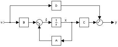
状态空间表示法即為一種將物理系統表示為一組輸入、輸出及狀態的數學模式,而輸入、輸出及狀態之間的關係可用許多一階微分方程來描述。
為了使數學模式不受輸入、輸出及狀態的個數所影響,輸入、輸出及狀態都會以向量的形式表示,而微分方程(若是線性非時變系統,可將微分方程轉變為代數方程)則會以矩陣的形式來表示。
状态空间表示法提供一種方便簡捷的方法來針對多輸入、多輸出的系統進行分析並建立模型。一般頻域的系統處理方式需限制在常係數,啟始條件為0的系統。而状态空间表示法對系統的係數及啟始條件沒有限制。
目录
1 状态变量
2 線性系統
2.1 連續非時變系統的例子
2.2 傳遞函數
2.3 可控制性
2.4 可觀察性
2.5 传递函数
2.6 正則实现
2.7 真分傳遞函數
2.8 反饋
2.9 有回授及目標值輸入
2.10 移動物體的範例
3 非線性系統
3.1 單擺的範例
4 相关条目
5 参考来源
6 延伸閱讀
状态变量
系統的狀態變數是指系統變數中,可以表示任一時間系統完整狀態的最小子集合。要表示一系統需要的狀態變數最小值n,通常也是該系統微分方程式的階數。若系統是以傳遞函數來表示,狀態變數的最小個數等於傳遞函數分母多項式的階數。在電路中狀態變數的個數常常就是電路中儲能元件(如電容器及電感器)的個數。
線性系統
一個有p{displaystyle p}


- x˙(t)=A(t)x(t)+B(t)u(t){displaystyle {dot {mathbf {x} }}(t)=A(t)mathbf {x} (t)+B(t)mathbf {u} (t)}
- y(t)=C(t)x(t)+D(t)u(t){displaystyle mathbf {y} (t)=C(t)mathbf {x} (t)+D(t)mathbf {u} (t)}


其中:
x(⋅){displaystyle mathbf {x} (cdot )}稱為狀態向量, x(t)∈Rn{displaystyle mathbf {x} (t)in mathbb {R} ^{n}}
;
y(⋅){displaystyle mathbf {y} (cdot )}稱為輸出向量, y(t)∈Rq{displaystyle mathbf {y} (t)in mathbb {R} ^{q}}
;
u(⋅){displaystyle mathbf {u} (cdot )}稱為輸入向量(或控制向量), u(t)∈Rp{displaystyle mathbf {u} (t)in mathbb {R} ^{p}}
;
A(⋅){displaystyle A(cdot )}稱為狀態矩陣, dim[A(⋅)]=n×n{displaystyle operatorname {dim} [A(cdot )]=ntimes n}
,
B(⋅){displaystyle B(cdot )}稱為輸入矩陣, dim[B(⋅)]=n×p{displaystyle operatorname {dim} [B(cdot )]=ntimes p}
,
C(⋅){displaystyle C(cdot )}稱為輸出矩陣, dim[C(⋅)]=q×n{displaystyle operatorname {dim} [C(cdot )]=qtimes n}
,
D(⋅){displaystyle D(cdot )}稱為前饋矩陣(若系統沒有直接從輸入到輸出的路徑,此矩陣為零矩陣), dim[D(⋅)]=q×p{displaystyle operatorname {dim} [D(cdot )]=qtimes p}
,
x˙(t):=ddtx(t){displaystyle {dot {mathbf {x} }}(t):={frac {operatorname {d} }{operatorname {d} t}}mathbf {x} (t)}.
通式中所有的矩陣均允許隨著時間而變化,此時所表示的就是線性時變系統。若表示的是线性非时变系统,则通式的矩陣都不會隨著時間變化。時間變數t{displaystyle t}


| 系統形式 | 状态空间模型 |
| 連續非時變系統 | x˙(t)=Ax(t)+Bu(t){displaystyle {dot {mathbf {x} }}(t)=Amathbf {x} (t)+Bmathbf {u} (t)}  y(t)=Cx(t)+Du(t){displaystyle mathbf {y} (t)=Cmathbf {x} (t)+Dmathbf {u} (t)}  |
| 連續時變系統 | x˙(t)=A(t)x(t)+B(t)u(t){displaystyle {dot {mathbf {x} }}(t)=mathbf {A} (t)mathbf {x} (t)+mathbf {B} (t)mathbf {u} (t)}  y(t)=C(t)x(t)+D(t)u(t){displaystyle mathbf {y} (t)=mathbf {C} (t)mathbf {x} (t)+mathbf {D} (t)mathbf {u} (t)}  |
| 離散非時變系統 | x(k+1)=Ax(k)+Bu(k){displaystyle mathbf {x} (k+1)=Amathbf {x} (k)+Bmathbf {u} (k)}  y(k)=Cx(k)+Du(k){displaystyle mathbf {y} (k)=Cmathbf {x} (k)+Dmathbf {u} (k)}  |
| 離散時變系統 | x(k+1)=A(k)x(k)+B(k)u(k){displaystyle mathbf {x} (k+1)=mathbf {A} (k)mathbf {x} (k)+mathbf {B} (k)mathbf {u} (k)}  y(k)=C(k)x(k)+D(k)u(k){displaystyle mathbf {y} (k)=mathbf {C} (k)mathbf {x} (k)+mathbf {D} (k)mathbf {u} (k)}  |
| 連續非時變系統 轉換到s域 | sX(s)=AX(s)+BU(s){displaystyle smathbf {X} (s)=Amathbf {X} (s)+Bmathbf {U} (s)}  Y(s)=CX(s)+DU(s){displaystyle mathbf {Y} (s)=Cmathbf {X} (s)+Dmathbf {U} (s)}  |
| 離散非時變系統 轉換到Z-域 | zX(z)=AX(z)+BU(z){displaystyle zmathbf {X} (z)=Amathbf {X} (z)+Bmathbf {U} (z)}  Y(z)=CX(z)+DU(z){displaystyle mathbf {Y} (z)=Cmathbf {X} (z)+Dmathbf {U} (z)}  |
連續非時變系統的例子
連續线性非时变系统的穩定性及響應特性可以由矩陣A的特徵值得到,也可以由系統對應的乘積型傳遞函數中得到。其型式如下所示:
- G(s)=k(s−z1)(s−z2)(s−z3)(s−p1)(s−p2)(s−p3)(s−p4){displaystyle {textbf {G}}(s)=k{frac {(s-z_{1})(s-z_{2})(s-z_{3})}{(s-p_{1})(s-p_{2})(s-p_{3})(s-p_{4})}}}

傳遞函數的分母等於sI−A{displaystyle sI-A}
λ(s)=|sI−A|{displaystyle mathbf {lambda } (s)=|sI-A|}.
其多項式的根即為矩陣A的特徵值,也是傳遞函數的极点。极点可以用來分析系統是否為指數穩定、臨界穩定或者根本不穩定。李雅普諾夫穩定性是另一種不需計算特徵值,也可以判斷穩定性的方式。
由傳遞函數的分子G(s){displaystyle {textbf {G}}(s)}
即使系統沒有內部穩定性,仍有可能是輸入輸出穩定系統。此情形時的不穩定极点和零點相消,為一個可去奇點。
傳遞函數
傳遞函數可用來描述線性非時變系統的特性。一個連續時間的線性非時變系統,可以用以下的方式,將其狀態空間表示式轉換為傳遞函數:
首先,對下式進行拉氏轉換
- x˙(t)=Ax(t)+Bu(t){displaystyle {dot {mathbf {x} }}(t)=Amathbf {x} (t)+Bmathbf {u} (t)}
可得到
- sX(s)=AX(s)+BU(s){displaystyle smathbf {X} (s)=Amathbf {X} (s)+Bmathbf {U} (s)}
再針對X(s){displaystyle mathbf {X} (s)}
- (sI−A)X(s)=BU(s){displaystyle (smathbf {I} -A)mathbf {X} (s)=Bmathbf {U} (s)}
- X(s)=(sI−A)−1BU(s){displaystyle mathbf {X} (s)=(smathbf {I} -A)^{-1}Bmathbf {U} (s)}


可以用此式來替換以下輸出方程式中的X(s){displaystyle mathbf {X} (s)}
- Y(s)=CX(s)+DU(s){displaystyle mathbf {Y} (s)=Cmathbf {X} (s)+Dmathbf {U} (s)}
結果如下
- Y(s)=C((sI−A)−1BU(s))+DU(s){displaystyle mathbf {Y} (s)=C((smathbf {I} -A)^{-1}Bmathbf {U} (s))+Dmathbf {U} (s)}

傳遞函數G(s){displaystyle mathbf {G} (s)}
- G(s)=Y(s)/U(s){displaystyle mathbf {G} (s)=mathbf {Y} (s)/mathbf {U} (s)}

因此可得到
- G(s)=C(sI−A)−1B+D{displaystyle mathbf {G} (s)=C(smathbf {I} -A)^{-1}B+D}

G(s){displaystyle mathbf {G} (s)}
若線性非時變系統有多個輸入及輸出時,其傳遞函數(也稱為傳遞矩陣)表示每一組輸入及輸出的關係,傳遞矩陣的每一個元素都是一組特定輸入及輸出的傳遞函數,不過多重輸入多重輸出(MIMO)的系統多仍使用状态空间的方式進行分析,較少使用傳遞函數或傳遞矩陣。
將一個系統由狀態空間表示式轉換為傳遞函數時,系統內部的資訊無法完整的轉換,可能系統表示為狀態空間表示式中在特定位置時會不穩定,但是用傳遞函數表示時卻是一個穩定的系統。
可控制性
一系統的狀態可控制性表示對於系統的一組初始狀態及一組終止狀態,存在一組輸入,使得此系統在有限時間內,可以由初始狀態轉移到終止狀態。一個連續线性时不变系统以状态空间表示時,系统若且唯若在以下秩的等式成立時才有可控制性
- rank[BABA2B...An−1B]=n{displaystyle operatorname {rank} {begin{bmatrix}B&AB&A^{2}B&...&A^{n-1}Bend{bmatrix}}=n}

(秩就是矩陣中線性獨立橫行的數目)
可觀察性
可觀察性是可以依一系統的輸出得知其系統內部的初始狀態。一系統的可觀察性及可控制性有數學上的對偶關係,可控制性是指可以利用輸入將系統由初始狀態轉換成任意的最終狀態,而可觀察性是指系統的輸出軌跡預測其初始狀態。
一個連續時間的線性非時變系統可觀察性,若且唯若下式成立:
- rank[CCA...CAn−1]=n{displaystyle operatorname {rank} {begin{bmatrix}C\CA\...\CA^{n-1}end{bmatrix}}=n}

传递函数
連續時間線性時不變的狀態空間模型可以用以下方式推導其传递函数:
首先,對下式進行拉普拉斯变换
- x˙(t)=Ax(t)+Bu(t){displaystyle {dot {mathbf {x} }}(t)=Amathbf {x} (t)+Bmathbf {u} (t)}
可得
- sX(s)−x(0)=AX(s)+BU(s).{displaystyle smathbf {X} (s)-mathbf {x} (0)=Amathbf {X} (s)+Bmathbf {U} (s).}

接下來,化簡X(s){displaystyle mathbf {X} (s)}
- (sI−A)X(s)=x(0)+BU(s),{displaystyle (smathbf {I} -A)mathbf {X} (s)=mathbf {x} (0)+Bmathbf {U} (s),}

因此
- X(s)=(sI−A)−1x(0)+(sI−A)−1BU(s).{displaystyle mathbf {X} (s)=(smathbf {I} -A)^{-1}mathbf {x} (0)+(smathbf {I} -A)^{-1}Bmathbf {U} (s).}

替換以下輸出方程中的X(s){displaystyle mathbf {X} (s)}
Y(s)=CX(s)+DU(s),{displaystyle mathbf {Y} (s)=Cmathbf {X} (s)+Dmathbf {U} (s),}可得
- Y(s)=C((sI−A)−1x(0)+(sI−A)−1BU(s))+DU(s).{displaystyle mathbf {Y} (s)=C((smathbf {I} -A)^{-1}mathbf {x} (0)+(smathbf {I} -A)^{-1}Bmathbf {U} (s))+Dmathbf {U} (s).}

传递函数 G(s){displaystyle mathbf {G} (s)}
- G(s)×U(s)=Y(s){displaystyle mathbf {G} (s)times mathbf {U} (s)=mathbf {Y} (s)}

比較Y(s){displaystyle mathbf {Y} (s)}
- G(s)=C(sI−A)−1B+D.{displaystyle mathbf {G} (s)=C(smathbf {I} -A)^{-1}B+D.}

可以看出G(s){displaystyle mathbf {G} (s)}
針對每一個輸入,有q{displaystyle q}
正則实现
任一個嚴格真分的傳遞函數,可以依以下的方式轉換為狀態空間的表示法(以下以一個4階、單一輸入及輸出的系統為例):
先將傳遞函數分子分母展開成以下的形式:
G(s)=n1s3+n2s2+n3s+n4s4+d1s3+d2s2+d3s+d4{displaystyle {textbf {G}}(s)={frac {n_{1}s^{3}+n_{2}s^{2}+n_{3}s+n_{4}}{s^{4}+d_{1}s^{3}+d_{2}s^{2}+d_{3}s+d_{4}}}}.
其分子分母的係數可以放進以下的狀態空間表示式中:
- x˙(t)=[−d1−d2−d3−d4100001000010]x(t)+[1000]u(t){displaystyle {dot {textbf {x}}}(t)={begin{bmatrix}-d_{1}&-d_{2}&-d_{3}&-d_{4}\1&0&0&0\0&1&0&0\0&0&1&0end{bmatrix}}{textbf {x}}(t)+{begin{bmatrix}1\0\0\0\end{bmatrix}}{textbf {u}}(t)}

y(t)=[n1n2n3n4]x(t){displaystyle {textbf {y}}(t)={begin{bmatrix}n_{1}&n_{2}&n_{3}&n_{4}end{bmatrix}}{textbf {x}}(t)}.
這種狀態空間的實現方式稱為“可控制正則型”(controllable canonical form),方便判斷系統的可控制性(控制輸入經過一連串的積分器後,即可影響每一個狀態),因此。
傳遞函數也可以轉換為以下的狀態空間表示式:
- x˙(t)=[−d1100−d2010−d3001−d4000]x(t)+[n1n2n3n4]u(t){displaystyle {dot {textbf {x}}}(t)={begin{bmatrix}-d_{1}&1&0&0\-d_{2}&0&1&0\-d_{3}&0&0&1\-d_{4}&0&0&0end{bmatrix}}{textbf {x}}(t)+{begin{bmatrix}n_{1}\n_{2}\n_{3}\n_{4}end{bmatrix}}{textbf {u}}(t)}

y(t)=[1000]x(t){displaystyle {textbf {y}}(t)={begin{bmatrix}1&0&0&0end{bmatrix}}{textbf {x}}(t)}.
這種狀態空間的實現方式稱為“可觀察正則型”(observable canonical form),方便判斷系統的可觀察性(輸出是經過狀態變數一連串積分後的輸出,因此可經由狀態變數影響系統的輸出)。
真分傳遞函數
若傳遞函數只是真分傳遞函數,不滿足嚴格真分的條件,可以將傳遞函數分為一嚴格真分數及常數的和,即可轉換為狀態空間的表示方式
- G(s)=GSP(s)+G(∞){displaystyle {textbf {G}}(s)={textbf {G}}_{SP}(s)+{textbf {G}}(infty )}

利用上一段的作法可以將嚴格真分傳遞函數轉換為正則型的狀態空間表示式。而常數部份可以轉換為y(t)=G(∞)u(t){displaystyle {textbf {y}}(t)={textbf {G}}(infty ){textbf {u}}(t)}
例如以下的真分傳遞函數
- G(s)=s2+3s+3s2+2s+1=s+2s2+2s+1+1{displaystyle {textbf {G}}(s)={frac {s^{2}+3s+3}{s^{2}+2s+1}}={frac {s+2}{s^{2}+2s+1}}+1}

其可控制正則型的實現如下
- x˙(t)=[−2−110]x(t)+[10]u(t){displaystyle {dot {textbf {x}}}(t)={begin{bmatrix}-2&-1\1&0\end{bmatrix}}{textbf {x}}(t)+{begin{bmatrix}1\0end{bmatrix}}{textbf {u}}(t)}

- y(t)=[12]x(t)+[1]u(t){displaystyle {textbf {y}}(t)={begin{bmatrix}1&2end{bmatrix}}{textbf {x}}(t)+{begin{bmatrix}1end{bmatrix}}{textbf {u}}(t)}

其輸出直接受到輸入的影響,原因就是因為傳遞函數的常數部份。
反饋

要為系統增加反饋,可以將輸出乘以一矩陣K,當作系統的輸入:u(t)=Ky(t){displaystyle mathbf {u} (t)=Kmathbf {y} (t)}
因此系統
- x˙(t)=Ax(t)+Bu(t){displaystyle {dot {mathbf {x} }}(t)=Amathbf {x} (t)+Bmathbf {u} (t)}
- y(t)=Cx(t)+Du(t){displaystyle mathbf {y} (t)=Cmathbf {x} (t)+Dmathbf {u} (t)}
可改寫為以下的形式
- x˙(t)=Ax(t)+BKy(t){displaystyle {dot {mathbf {x} }}(t)=Amathbf {x} (t)+BKmathbf {y} (t)}
- y(t)=Cx(t)+DKy(t){displaystyle mathbf {y} (t)=Cmathbf {x} (t)+DKmathbf {y} (t)}


求解y(t){displaystyle mathbf {y} (t)}
- x˙(t)=(A+BK(I−DK)−1C)x(t){displaystyle {dot {mathbf {x} }}(t)=left(A+BKleft(I-DKright)^{-1}Cright)mathbf {x} (t)}
- y(t)=(I−DK)−1Cx(t){displaystyle mathbf {y} (t)=left(I-DKright)^{-1}Cmathbf {x} (t)}


此作法的好處是整個系統的特性不止是由矩陣A的特徵值決定,也可以由K的適當設定及(A+BK(I−DK)−1C){displaystyle left(A+BKleft(I-DKright)^{-1}Cright)}
有一種常見的簡化法是令矩陣D為零矩陣,矩陣C為單位矩陣,因此方程式可以簡化為以下的形式:
- x˙(t)=(A+BK)x(t){displaystyle {dot {mathbf {x} }}(t)=left(A+BKright)mathbf {x} (t)}
- y(t)=x(t){displaystyle mathbf {y} (t)=mathbf {x} (t)}


需進行特徵值分解的矩陣縮小為A+BK{displaystyle A+BK}
有回授及目標值輸入

回授信號也可以再加上目標值輸入r(t){displaystyle r(t)}

- x˙(t)=Ax(t)+Bu(t){displaystyle {dot {mathbf {x} }}(t)=Amathbf {x} (t)+Bmathbf {u} (t)}
- y(t)=Cx(t)+Du(t){displaystyle mathbf {y} (t)=Cmathbf {x} (t)+Dmathbf {u} (t)}
變成以下的形式
- x˙(t)=Ax(t)−BKy(t)+Br(t){displaystyle {dot {mathbf {x} }}(t)=Amathbf {x} (t)-BKmathbf {y} (t)+Bmathbf {r} (t)}
- y(t)=Cx(t)−DKy(t)+Dr(t){displaystyle mathbf {y} (t)=Cmathbf {x} (t)-DKmathbf {y} (t)+Dmathbf {r} (t)}


求解y(t){displaystyle mathbf {y} (t)}
- x˙(t)=(A−BK(I+DK)−1C)x(t)+B(I−K(I+DK)−1D)r(t){displaystyle {dot {mathbf {x} }}(t)=left(A-BKleft(I+DKright)^{-1}Cright)mathbf {x} (t)+Bleft(I-Kleft(I+DKright)^{-1}Dright)mathbf {r} (t)}
- y(t)=(I+DK)−1Cx(t)+(I+DK)−1Dr(t){displaystyle mathbf {y} (t)=left(I+DKright)^{-1}Cmathbf {x} (t)+left(I+DKright)^{-1}Dmathbf {r} (t)}


一個常見的簡化是令矩陣D為零矩陣,方程式可簡化為以下的形式
- x˙(t)=(A−BKC)x(t)+Br(t){displaystyle {dot {mathbf {x} }}(t)=left(A-BKCright)mathbf {x} (t)+Bmathbf {r} (t)}
- y(t)=Cx(t){displaystyle mathbf {y} (t)=Cmathbf {x} (t)}


移動物體的範例
以下以物體的一維移動來作為範例。
考慮一物體在一平面上水平移動,物體和牆壁之間有彈簧相連接,依牛頓第二運動定律,其受力如下
- my¨(t)=u(t)−k1y˙(t)−k2y(t){displaystyle m{ddot {y}}(t)=u(t)-k_{1}{dot {y}}(t)-k_{2}y(t)}

其中
y(t){displaystyle y(t)}為位置,y˙(t){displaystyle {dot {y}}(t)}
及y¨(t){displaystyle {ddot {y}}(t)}
分別是速度及加速度
u(t){displaystyle u(t)}為施力
k1{displaystyle k_{1}}為粘滞摩擦係數
k2{displaystyle k_{2}}為彈簧的彈性常數
m{displaystyle m}為物體的質量
其狀態方程式可以下式表示
- [x1˙(t)x2˙(t)]=[01−k2m−k1m][x1(t)x2(t)]+[01m]u(t){displaystyle left[{begin{matrix}mathbf {dot {x_{1}}} (t)\mathbf {dot {x_{2}}} (t)end{matrix}}right]=left[{begin{matrix}0&1\-{frac {k_{2}}{m}}&-{frac {k_{1}}{m}}end{matrix}}right]left[{begin{matrix}mathbf {x_{1}} (t)\mathbf {x_{2}} (t)end{matrix}}right]+left[{begin{matrix}0\{frac {1}{m}}end{matrix}}right]mathbf {u} (t)}
- y(t)=[10][x1(t)x2(t)]{displaystyle mathbf {y} (t)=left[{begin{matrix}1&0end{matrix}}right]left[{begin{matrix}mathbf {x_{1}} (t)\mathbf {x_{2}} (t)end{matrix}}right]}
![left[{begin{matrix}{mathbf {{dot {x_{1}}}}}(t)\{mathbf {{dot {x_{2}}}}}(t)end{matrix}}right]=left[{begin{matrix}0&1\-{frac {k_{2}}{m}}&-{frac {k_{1}}{m}}end{matrix}}right]left[{begin{matrix}{mathbf {x_{1}}}(t)\{mathbf {x_{2}}}(t)end{matrix}}right]+left[{begin{matrix}0\{frac {1}{m}}end{matrix}}right]{mathbf {u}}(t)](https://wikimedia.org/api/rest_v1/media/math/render/svg/0bde243f9d17f91b1d03020e9559e8120fae677f)
![{mathbf {y}}(t)=left[{begin{matrix}1&0end{matrix}}right]left[{begin{matrix}{mathbf {x_{1}}}(t)\{mathbf {x_{2}}}(t)end{matrix}}right]](https://wikimedia.org/api/rest_v1/media/math/render/svg/089622c024d88e55fb7da811b54574235a1af4a1)
其中
x1(t){displaystyle x_{1}(t)}為物體的位置
x2(t)=x1˙(t){displaystyle x_{2}(t)={dot {x_{1}}}(t)}為物體的速度
x2˙(t)=x1¨(t){displaystyle {dot {x_{2}}}(t)={ddot {x_{1}}}(t)}為物體的加速度
- 輸出y(t){displaystyle mathbf {y} (t)}
依可控制性測試,結果為
- [BAB]=[[01m][01−k2m−k1m][01m]]=[01m1mk1m2]{displaystyle left[{begin{matrix}B&ABend{matrix}}right]=left[{begin{matrix}left[{begin{matrix}0\{frac {1}{m}}end{matrix}}right]&left[{begin{matrix}0&1\-{frac {k_{2}}{m}}&-{frac {k_{1}}{m}}end{matrix}}right]left[{begin{matrix}0\{frac {1}{m}}end{matrix}}right]end{matrix}}right]=left[{begin{matrix}0&{frac {1}{m}}\{frac {1}{m}}&{frac {k_{1}}{m^{2}}}end{matrix}}right]}
![left[{begin{matrix}B&ABend{matrix}}right]=left[{begin{matrix}left[{begin{matrix}0\{frac {1}{m}}end{matrix}}right]&left[{begin{matrix}0&1\-{frac {k_{2}}{m}}&-{frac {k_{1}}{m}}end{matrix}}right]left[{begin{matrix}0\{frac {1}{m}}end{matrix}}right]end{matrix}}right]=left[{begin{matrix}0&{frac {1}{m}}\{frac {1}{m}}&{frac {k_{1}}{m^{2}}}end{matrix}}right]](https://wikimedia.org/api/rest_v1/media/math/render/svg/8085052653d9c3f6548abce458f14b47264c544f)
對所有非零的k1{displaystyle k_{1}}
依可觀察性測試,結果為
- [CCA]=[[10][10][01−k2m−k1m]]=[1001]{displaystyle left[{begin{matrix}C\CAend{matrix}}right]=left[{begin{matrix}left[{begin{matrix}1&0end{matrix}}right]\left[{begin{matrix}1&0end{matrix}}right]left[{begin{matrix}0&1\-{frac {k_{2}}{m}}&-{frac {k_{1}}{m}}end{matrix}}right]end{matrix}}right]=left[{begin{matrix}1&0\0&1end{matrix}}right]}
![left[{begin{matrix}C\CAend{matrix}}right]=left[{begin{matrix}left[{begin{matrix}1&0end{matrix}}right]\left[{begin{matrix}1&0end{matrix}}right]left[{begin{matrix}0&1\-{frac {k_{2}}{m}}&-{frac {k_{1}}{m}}end{matrix}}right]end{matrix}}right]=left[{begin{matrix}1&0\0&1end{matrix}}right]](https://wikimedia.org/api/rest_v1/media/math/render/svg/379549fbd631c3d00cff027b1208378f396a65e0)
對所有非零的k1{displaystyle k_{1}}
因此,此系統具有可控制性及可觀察性。
非線性系統
以下將狀態空間模型以函數的形式來表示。
- x˙(t)=f(t,x(t),u(t)){displaystyle mathbf {dot {x}} (t)=mathbf {f} (t,x(t),u(t))}
- y(t)=h(t,x(t),u(t)){displaystyle mathbf {y} (t)=mathbf {h} (t,x(t),u(t))}


第一個方程式為狀態方程式,第二個方程式為輸出方程式。
此表示法可以表示線性系統及非線性系統。若函數f(⋅,⋅,⋅){displaystyle f(cdot ,cdot ,cdot )}
若系統沒有外力(沒有輸入項),則以上方程式中的u(t){displaystyle u(t)}
單擺的範例
單擺即為一個非線性系統的例子。
- mlθ¨(t)=−mgsinθ(t)−klθ˙(t){displaystyle ml{ddot {theta }}(t)=-mgsin theta (t)-kl{dot {theta }}(t)}

其中
θ(t){displaystyle theta (t)}為單擺偏離垂線的角度
m{displaystyle m}
g{displaystyle g}為重力加速度
k{displaystyle k}
l{displaystyle l}為單擺的半徑(以質量m{displaystyle m}
其狀態方程式為
- x1˙(t)=x2(t){displaystyle {dot {x_{1}}}(t)=x_{2}(t)}
- x2˙(t)=−glsinx1(t)−kmx2(t){displaystyle {dot {x_{2}}}(t)=-{frac {g}{l}}sin {x_{1}}(t)-{frac {k}{m}}{x_{2}}(t)}


其中
x1(t)=θ(t){displaystyle x_{1}(t)=theta (t)}為單擺的角度
x2(t)=x1˙(t){displaystyle x_{2}(t)={dot {x_{1}}}(t)}
x2˙=x1¨{displaystyle {dot {x_{2}}}={ddot {x_{1}}}}為單擺的角加速度
其狀態方程式可寫成以下的形式
- x˙(t)=(x1˙(t)x2˙(t))=f(t,x(t))=(x2(t)−glsinx1(t)−kmx2(t)).{displaystyle {dot {x}}(t)=left({begin{matrix}{dot {x_{1}}}(t)\{dot {x_{2}}}(t)end{matrix}}right)=mathbf {f} (t,x(t))=left({begin{matrix}x_{2}(t)\-{frac {g}{l}}sin {x_{1}}(t)-{frac {k}{m}}{x_{2}}(t)end{matrix}}right).}

一系統的機械平衡點或駐點為x˙=0{displaystyle {dot {x}}=0}
- (x1x2)=(nπ0){displaystyle left({begin{matrix}x_{1}\x_{2}end{matrix}}right)=left({begin{matrix}npi \0end{matrix}}right)}

其中n為整數。
相关条目
- 离散化
相空間:物理學和數學中有關相空間(例如連續的狀態空間)的資訊。
狀態空間 (計算機科學):計算機科學中有關狀態空間的資訊。
機率空間:機率中關於狀態空間的資訊。- 卡尔曼滤波
参考来源
^ I.J.Nagrath, M.Goral. Control System Engineering. Wiley Eastern Limited. 1985: 450. ISBN 9579590532.
^ 朱福喜,朱三元,伍春香. 《人工智能基础教程》. 清华大学出版社. 2006年. ISBN 9787302125778.
延伸閱讀
.mw-parser-output .refbegin{font-size:90%;margin-bottom:0.5em}.mw-parser-output .refbegin-hanging-indents>ul{list-style-type:none;margin-left:0}.mw-parser-output .refbegin-hanging-indents>ul>li,.mw-parser-output .refbegin-hanging-indents>dl>dd{margin-left:0;padding-left:3.2em;text-indent:-3.2em;list-style:none}.mw-parser-output .refbegin-100{font-size:100%}
- Antsaklis, P.J. and Michel, A.N. 2007. A Linear Systems Primer, Birkhauser. (ISBN 978-0-8176-4434-50)
- Chen, Chi-Tsong 1999. Linear System Theory and Design, 3rd. ed., Oxford University Press (ISBN 978-0-19-511777-6)
- Khalil, Hassan K. 2001 Nonlinear Systems, 3rd. ed., Prentice Hall (ISBN 978-0-13-067389-3)
- Nise, Norman S. 2004. Control Systems Engineering, 4th ed., John Wiley & Sons, Inc. (ISBN 978-0-471-44577-7)
- Hinrichsen, Diederich and Pritchard, Anthony J. 2005. Mathematical Systems Theory I, Modelling, State Space Analysis, Stability and Robustness. Springer. (ISBN 978-3-540-44125-0)
- Sontag, Eduardo D. 1999. Mathematical Control Theory: Deterministic Finite Dimensional Systems. Second Edition. Springer. (ISBN 978-0-387-98489-6) (available free online)
- Friedland, Bernard. 2005. Control System Design: An Introduction to State Space Methods. Dover. (ISBN 978-0-486-44278-5).
- Zadeh, Lofti A. and Desoer, Charles A. 1979. Linear System Theory, Krieger Pub Co. (ISBN 978-0-88275-809-1)
| ||||||||||||||||||||||||||||||||


Comments
Post a Comment